Home / Past papers / MLT End Term / this paper
IIT M IMPROVEMENT AN EXAM QDD3 01 - 01 Sep 2024
Elapsed 00:00



- 1
- 2
- 3
- 6





Match the characteristics given below with the appropriate ensemble technique. 1. Decision stumps 2. Deep decision trees 3. Parallel execution 4. Sequential execution
- Bagging → (2), (3); Boosting → (1), (4)
- Bagging → (1), (4); Boosting → (2), (3)
- Bagging → (1), (3); Boosting → (2), (4)
- Bagging → (2), (4); Boosting → (1), (3)









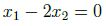
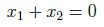


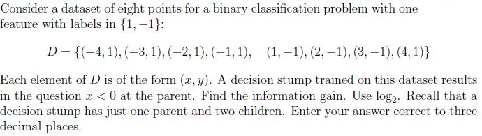
- 0.75
- 0.25
- 0.5
- 0.15





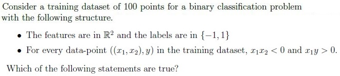
- The dataset is linearly separable with a positive margin.
- The perceptron algorithm will terminate after a finite number of iterationswhen trained on this dataset.
- The dataset is linearly separable, but the margin may be zero.
- The dataset is not linearly separable.


Comprehension passage - the questions below it refer to this

The weight vector output by the perceptron algorithm can be expressed as a linear combination of the data-points where the coefficients of the linear combination are integers.
- TRUE
- FALSE

- TRUE
- FALSE
If a soft-margin SVM is trained on this dataset, the optimal weight vector it returns will be the same as the one returned by a hard-margin SVM, irrespective of the value of the hyperparameter C.
- TRUE
- FALSE
Comprehension passage - the questions below it refer to this
Based on the above data, answer the given subquestions.
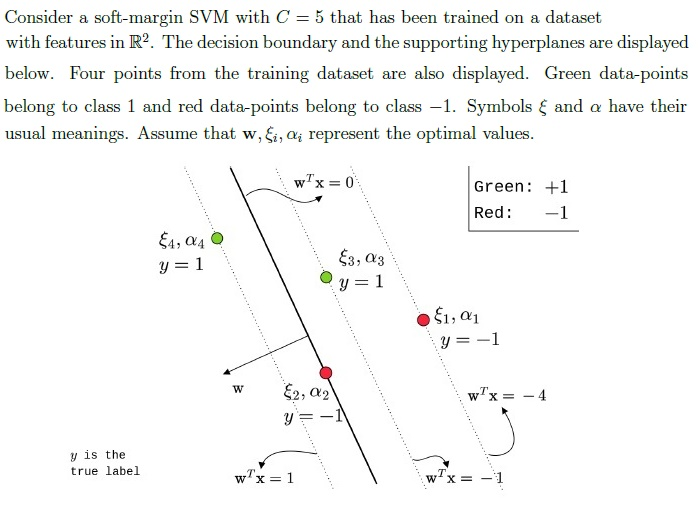





Comprehension passage - the questions below it refer to this
Based on the above data, answer the given subquestions.
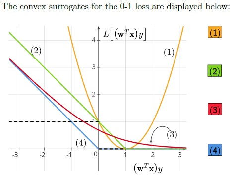
Enter the number corresponding to the logistic loss.
Enter the number corresponding to the (SVM) hinge loss.
Enter the number corresponding to the perceptron loss.
Enter the number corresponding to the squared loss.





Comprehension passage - the questions below it refer to this
Based on the above data, answer the given subquestions.
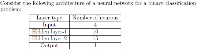
How many learnable parameters does this network have? Ignore the biases in the computation.
What is the most appropriate choice of activation function for the output layer if the binary cross-entropy loss is used?
- Sigmoid
- Linear
- ReLU
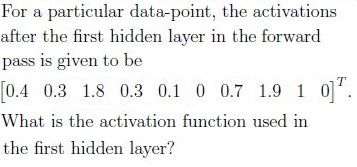
- ReLU
- Sigmoid
Answer key
- Q1 (MCQ, 2 marks): A
- Q2 (MCQ, 3 marks): C
- Q3 (MCQ, 3 marks): A
- Q4 (MCQ, 3 marks): A
- Q5 (MCQ, 3 marks): B
- Q6 (MCQ, 3 marks): A
- Q7 (MCQ, 3 marks): A
- Q8 (MCQ, 3 marks): A
- Q9 (MSQ, 3 marks): A, B
- Q10 (MSQ, 3 marks): A, B
- Q11 (SA, 3 marks): 10
- Q12 (SA, 3 marks): 0.75
- Q13 (SA, 3 marks): 0.50 to 0.60
- Q14 (MCQ, 1 marks): A
- Q15 (MCQ, 1 marks): B
- Q16 (MCQ, 1 marks): B
- Q17 (SA, 0.5 marks): 0
- Q18 (SA, 0.5 marks): 1
- Q19 (SA, 0.5 marks): 2
- Q20 (SA, 0.5 marks): 0
- Q21 (SA, 0.5 marks): 5
- Q22 (SA, 0.5 marks): -1
- Q23 (SA, 0.5 marks): 3
- Q24 (SA, 0.5 marks): 2
- Q25 (SA, 0.5 marks): 4
- Q26 (SA, 0.5 marks): 1
- Q27 (MCQ, 1 marks): A
- Q28 (SA, 1 marks): 205
- Q29 (MCQ, 1 marks): A
- Q30 (MCQ, 1 marks): A
Concepts this paper tests
Auto-generated summary from the source site. Handy as a checklist; the lessons above explain each idea from scratch.
Here’s a structured summary of core topics, concepts, principles, and equations for the Diploma-Level Machine Learning Techniques exam, along with Mermaid knowledge graphs to visualize relationships.
1. Core Topics & Key Concepts
A. Linear Regression & Gradient Descent
Key Concepts:
- Sum of Squared Errors (SSE): , where .
- Gradient of SSE (for a single data point): . (From Q2: Correct option was missing, but the gradient is derived from .)
Ridge Regression (L2 Regularization): .
Effect of :
- Small (e.g., ): Overfitting (high variance).
- Large (e.g., ): Underfitting (high bias).
(From Q4: Correct answer was A.)
Equations:
- SSE Gradient (Vector Form): .
- Ridge Regression Update: .
B. Principal Component Analysis (PCA)
Key Concepts:
- Covariance Matrix : (for centered data).
- Principal Components: Eigenvectors of , sorted by eigenvalues (variance).
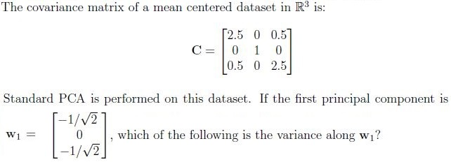
- Variance along a Principal Component : . (From Q3: Given , variance = 3.)
Equations:
- Variance Calculation: .
- Projection onto PC: .
C. Support Vector Machines (SVM)
Key Concepts:
Hard-Margin SVM:
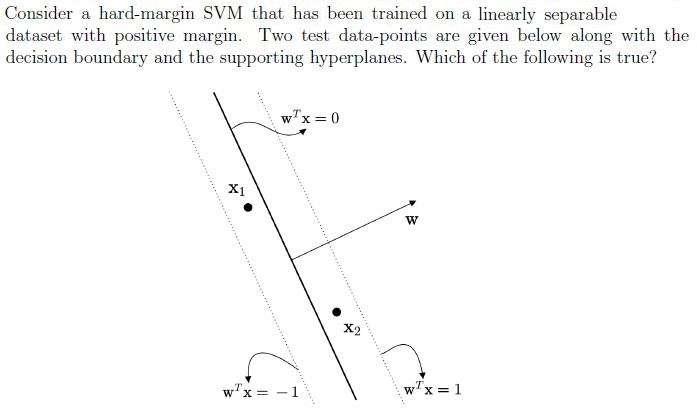
- Decision boundary: .
- Supporting hyperplanes: .
- Margin: . (From Q12: Margin = 0.2 ⇒ .)
Soft-Margin SVM:
- Allows misclassification with slack variables .
- Objective: .
- Kernel Trick: . (From Q10: Valid kernels include polynomial and RBF.)
- Support Vectors: Points with . (From Q16: If , is a support vector.)
Equations:
- Hard-Margin Constraint: .
- Soft-Margin Constraint: , .
- Kernel SVM Dual Problem: .
D. Ensemble Methods
Key Concepts:
Bagging (Bootstrap Aggregating):
- Trains models in parallel on bootstrapped samples.
- Uses deep trees (high variance, low bias).
- Example: Random Forest.
Boosting:
- Trains models sequentially, correcting errors.
- Uses weak learners (e.g., decision stumps).
- Example: AdaBoost, Gradient Boosting.
(From Q5: Bagging → (2, 3); Boosting → (1, 4).)
E. Naive Bayes
Key Concepts:
- Class Conditional Independence: . (From Q7: Correct answer was A.)
Equations:
- Posterior Probability: .
F. Clustering (k-Means)
Key Concepts:
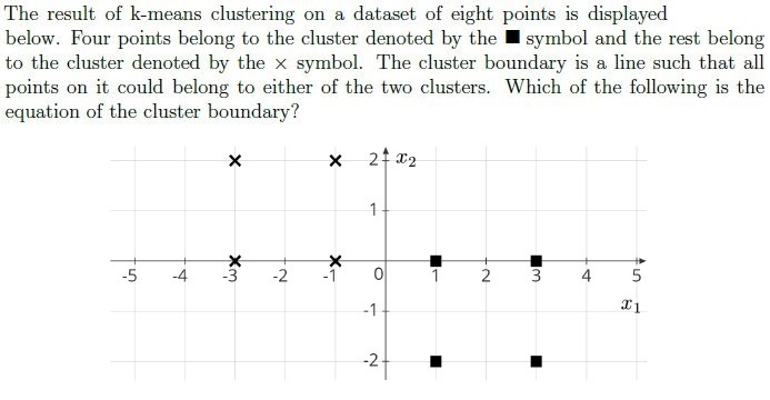
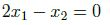
- Cluster Boundary: Perpendicular bisector between centroids. (From Q8: Boundary equation was .)
Equations:
- Centroid Update: .
G. Logistic Regression
Key Concepts:
- Sigmoid Function: , where .
- Probability Symmetry: , . (From Q9: .)
Equations:
- Logistic Loss: .
H. Decision Trees & Information Gain
Key Concepts:
- Entropy: .
- Information Gain: . (From Q14: IG = 0.594 for the split .)
Equations:
- Binary Entropy: .
I. Neural Networks
Key Concepts:
- Learnable Parameters: , where = neurons in layer . (From Q29: 4→10→15→1 ⇒ 205 params.)
Activation Functions:
- Output Layer (Binary Classification): Sigmoid (with cross-entropy loss). (From Q30: Correct answer was A.)
- Hidden Layers: ReLU (from Q31, since activations include zeros).
Equations:
- ReLU: .
- Sigmoid: .
J. Loss Functions
Key Concepts:
Convex Surrogates for 0-1 Loss:
- Logistic Loss: .
- Hinge Loss (SVM): .
- Perceptron Loss: .
- Squared Loss: .
(From Q24–Q27: Match colors to curves.)
- Intersection of Logistic & Hinge Loss: Occurs at . (From Q28: Correct answer was A.)
Equations:
- Hinge Loss: .
- Logistic Loss: .
K. Bayesian Learning
Key Concepts:
Beta-Binomial Conjugacy:
- Prior: .
- Posterior: .
(From Q13: Posterior = Beta(15, 5) ⇒ .)
Equations:
- Beta Expected Value: .
Graph 2: Ensemble Methods
Graph 3: Dimensionality Reduction & Clustering
Graph 4: Neural Networks
Graph 5: Loss Functions
3. Summary of Key Equations
| Topic | Equation |
|---|---|
| SSE Gradient | |
| Ridge Regression | |
| PCA Variance | |
| SVM Margin | |
| Logistic Regression | |
| Information Gain | |
| Neural Network Params | |
| Beta Posterior | |
| Hinge Loss | |
| Logistic Loss |