Home / Past papers / MLT Quiz 1 / this paper

IIT M IMPROVEMENT AN EXAM QIE4 26 Oct - 26 Oct 2025

MLT Quiz 114 questions40 marks6 SA · 5 MSQ · 3 MCQImprovement / afternoon / QIE4

Elapsed 00:00

Q1MSQ2 marksselect all that apply

Which among the following is true with respect to the Lloyds’ algorithm?

It always converges.
It may fail to converge for an initialization while it may converge for otherinitialization.
It is sensitive to outliers.
The solution produced is always the optimal.

Q2MSQ4 marksselect all that apply

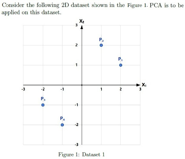
There will be 50 non-zero eigenvalues of the covariance matrix.
There will be 6 non-zero eigenvalues of the covariance matrix.
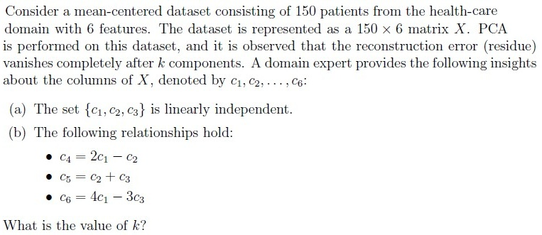
Using the first 5 principal components, the dataset can be reconstructed withzero residue.
The variance captured by the top 6 principal components equals the totalvariance of the dataset.

Q3MSQ4 marksselect all that apply

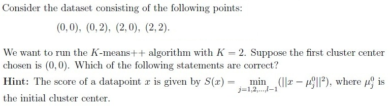
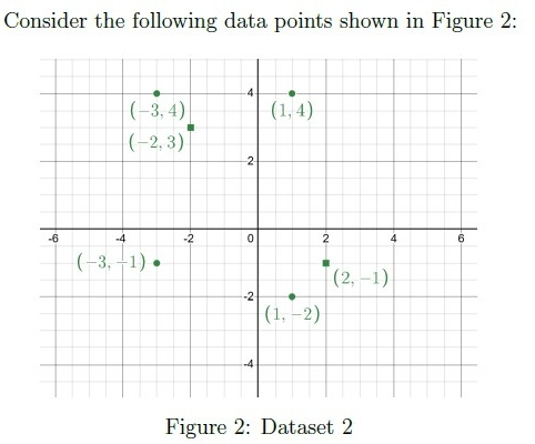
The points (0, 2), (2, 0), and (2, 2) have the equal probability of being chosen asthe second cluster center.
The probability of selecting (2, 2) as the second cluster center is twice that ofselecting (0, 2).
If (2, 2) is chosen as the second cluster center, the algorithm will alwaysconverge in one iteration.
The tie-breaking rule will affect the final cluster centers.

Q4MSQ4 marksselect all that apply

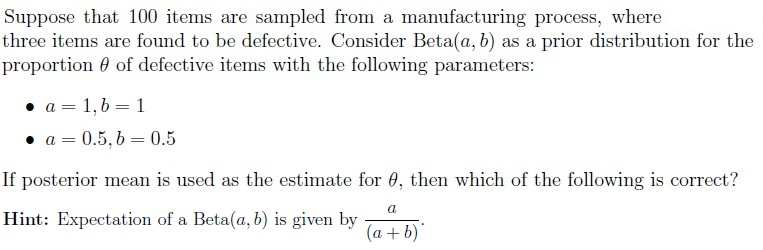
Posterior mean for Beta(1, 1) is 0.039.
Posterior mean for Beta(1, 1) is 0.03.
Posterior mean for Beta(0.5, 0.5) is 0.025.
Posterior mean for Beta(0.5, 0.5) is 0.034.

Q5MSQ3 marksselect all that apply

Which of the following are valid kernel functions? Select all that apply.

Q6SA3 marks

Your numeric answer:

Q7SA3 marks

Your numeric answer:

Comprehension passage - the questions below it refer to this

Based on the above data, answer the given subquestions. question figure

Q8MCQ2 marks

What is the covariance matrix of the dataset?

Q9SA2 marks

If standard PCA is performed on this dataset, what is the variance along the first principal component? Enter the answer correct to one decimal place.

Your numeric answer:

Q10SA2 marks

If standard PCA is performed on this dataset, what is the variance along the second principal component? Enter the answer correct to one decimal place.

Your numeric answer:

Comprehension passage - the questions below it refer to this

Based on the above data, answer the given subquestions. question figure

Q11MCQ3 marks

Q12SA3 marks

Your numeric answer:

Comprehension passage - the questions below it refer to this

Based on the above data, answer the given subquestions. question figure

Q13MCQ3 marks

Perform K-means clustering with K = 2 and initial cluster centers at (−2, 3) and (2,−1). What are the final means of clusters after convergence?

Q14SA2 marks

Suppose we introduce a new data point (0, 0) to the existing dataset and perform K means with the same initial cluster centers. How many iterations would it require now for convergence?

Your numeric answer:

Answer key

Q1 (MSQ, 2 marks): A, C
Q2 (MSQ, 4 marks): B, D
Q3 (MSQ, 4 marks): B, C, D
Q4 (MSQ, 4 marks): A, D
Q5 (MSQ, 3 marks): A, B, D
Q6 (SA, 3 marks): 3
Q7 (SA, 3 marks): 0.45 to 0.50
Q8 (MCQ, 2 marks): B
Q9 (SA, 2 marks): 4.5
Q10 (SA, 2 marks): 0.5
Q11 (MCQ, 3 marks): B
Q12 (SA, 3 marks): 0.64 to 0.68
Q13 (MCQ, 3 marks): A
Q14 (SA, 2 marks): 1

Concepts this paper tests

Auto-generated summary from the source site. Handy as a checklist; the lessons above explain each idea from scratch.

Here’s a structured summary of core topics, concepts, principles, and equations for the Diploma-Level Machine Learning Techniques exam, along with Mermaid knowledge graphs to visualize relationships.

1. Core Topics & Concepts

A. Clustering (K-Means, K-Means++, Lloyd’s Algorithm, EM for GMM)

K-Means & K-Means++
- Lloyd’s Algorithm (Standard K-Means):
  - Convergence: Always converges (monotonically decreases objective function, but may reach local minima).
  - Sensitivity: Sensitive to outliers (uses Euclidean distance).
  - Optimality: Does not guarantee global optimum (depends on initialization).
  - Initialization: K-Means++ improves initialization by selecting centers probabilistically based on distances.
    - Score for K-Means++:

S(x) = \min_{j=1,\ldots,l-1} \|x - \mu_j^0\|^2

(Probability of selecting a point as next center ∝ $S(x)$ ).

Convergence Criteria: Assignments and centroids stabilize (no change between iterations).

Gaussian Mixture Models (GMM) & EM Algorithm
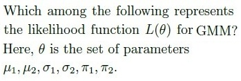
- Likelihood Function for GMM:

L(\theta) = \prod_{i=1}^n \sum_{k=1}^K \pi_k \cdot \mathcal{N}(x_i | \mu_k, \sigma_k^2)

where $\theta = \{\pi_k, \mu_k, \sigma_k^2\}_{k=1}^K$ .

EM Steps:
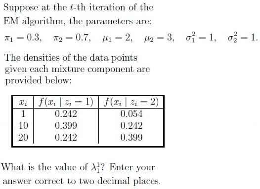
- E-Step: Compute responsibilities ( $\lambda_{ik}$ ):

\lambda_{ik} = \frac{\pi_k \mathcal{N}(x_i | \mu_k, \sigma_k^2)}{\sum_{j=1}^K \pi_j \mathcal{N}(x_i | \mu_j, \sigma_j^2)}

M-Step: Update parameters:

\mu_k = \frac{\sum_i \lambda_{ik} x_i}{\sum_i \lambda_{ik}}, \quad \sigma_k^2 = \frac{\sum_i \lambda_{ik} (x_i - \mu_k)^2}{\sum_i \lambda_{ik}}, \quad \pi_k = \frac{\sum_i \lambda_{ik}}{n}

B. Dimensionality Reduction (PCA)

Principal Component Analysis (PCA):
- Goal: Project data into a lower-dimensional subspace while maximizing variance.
- Steps:
  1. Center the data (subtract mean).
  2. Compute covariance matrix $C = \frac{1}{n-1} X^T X$ .
  3. Eigen decomposition: $C = V \Lambda V^T$ (eigenvectors $V$ , eigenvalues $\Lambda$ ).
  4. Select top- $k$ eigenvectors (principal components) with largest eigenvalues.
- Variance Captured:
  - Total variance = sum of all eigenvalues.
  - Variance of $i$ -th PC = $\lambda_i$ .
  - Proportion of variance explained by first $k$ PCs:

\text{Proportion} = \frac{\sum_{i=1}^k \lambda_i}{\sum_{i=1}^d \lambda_i}

Reconstruction Error: Zero if $k = \text{rank}(X)$ . For a dataset in a $k$ -dimensional subspace, only $k$ eigenvalues are non-zero.

Key Properties:
- If data lies in a $k$ -dimensional subspace of $\mathbb{R}^d$ , the first $k$ PCs capture all variance.
- Eigenvalues of $X^T X$ represent variances along PCs.

C. Bayesian Statistics (Beta-Binomial Model)

Beta Distribution as Prior for Proportion $\theta$ :
- Prior: $\theta \sim \text{Beta}(a, b)$ .
- Posterior (after observing $x$ successes in $n$ trials):

\theta | \text{data} \sim \text{Beta}(a + x, b + n - x)

Posterior Mean (Estimate for $\theta$ ):

\mathbb{E}[\theta | \text{data}] = \frac{a + x}{a + b + n}

D. Kernel Methods

Valid Kernel Functions (Mercer’s Condition):
- Gaussian (RBF) Kernel:

K(x, y) = \exp\left(-\frac{\|x - y\|^2}{2\sigma^2}\right)

Polynomial Kernel:

K(x, y) = (x \cdot y + c)^d, \quad c \geq 0, d \in \mathbb{N}

Laplacian Kernel:

K(x, y) = \exp\left(-\frac{\|x - y\|}{\sigma}\right)

Invalid Kernel: $K(x, y) = |x - y|$ (not positive semi-definite).

2. Key Equations

Topic	Equation
K-Means++ Score	$S(x) = \min_{j} \\|x - \mu_j^0\\|^2$
GMM Likelihood	$L(\theta) = \prod_i \sum_k \pi_k \mathcal{N}(x_i \| \mu_k, \sigma_k^2)$
PCA Variance	$\text{Variance of PC}_i = \lambda_i$
PCA Proportion	$\frac{\sum_{i=1}^k \lambda_i}{\sum_{i=1}^d \lambda_i}$
Beta Posterior Mean	$\mathbb{E}[\theta \| \text{data}] = \frac{a + x}{a + b + n}$
Gaussian Kernel	$K(x, y) = \exp\left(-\frac{\\|x - y\\|^2}{2\sigma^2}\right)$
Polynomial Kernel	$K(x, y) = (x \cdot y + c)^d$

Graph 2: Dimensionality Reduction (PCA)

Graph 3: Bayesian Statistics (Beta-Binomial)

Graph 4: Kernel Methods

4. Exam-Specific Insights

PCA:
- If data lies in a $k$ -dimensional subspace, only $k$ eigenvalues are non-zero.
- Reconstruction error is zero if $k = \text{rank}(X)$ .
- Example: For 5000 points in $\mathbb{R}^{50}$ lying in a 6D subspace, the first 6 PCs capture all variance.

K-Means:
- Lloyd’s algorithm always converges but may not find the global optimum.
- K-Means++ reduces sensitivity to initialization by spreading out initial centers.

GMM:
- Likelihood involves a product of sums (not sums of products).
- Responsibilities ( $\lambda_{ik}$ ) are soft assignments (unlike hard assignments in K-Means).

Beta-Binomial:
- Posterior mean is a weighted average of prior mean and observed proportion.
- Example: For $\text{Beta}(1,1)$ (uniform prior) and 3 defects in 100 samples:

\mathbb{E}[\theta] = \frac{1 + 3}{1 + 1 + 100} = 0.039

Kernels:
- Valid kernels must satisfy Mercer’s condition (positive semi-definite).
- Invalid kernel: $K(x, y) = |x - y|$ (not PSD).