Home / Past papers / MLT End Term / this paper
2023 Dec24: IIT M AN EXAM ADD4 - 24 Dec 2023
Elapsed 00:00



Comprehension passage - the questions below it refer to this
Based on the above data, answer the given subquestions.
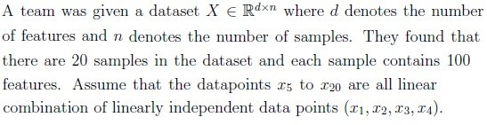
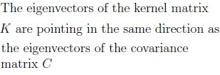
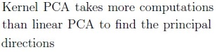
Suppose the team applies linear PCA on the dataset and reconstructs the data points with zero error using k principal components (directions). For which value of k the reconstruction error would become zero?
- 1
- 2
- 3
- 4
- 10
- 100
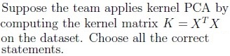
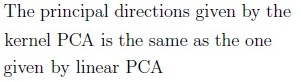
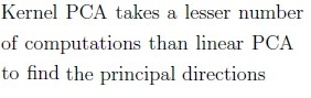
Consider Lloyd’s algorithm used for k-means clustering and choose the correct statements:
- K-means algorithm may get stuck at local minima.
- It guarantees finding the optimal clustering(global minima) in every run.
- If the resources are limited and the data set is huge, it will be good to prefer K-means over K-means++.
- In practice, k should be as large as possible.
Comprehension passage - the questions below it refer to this
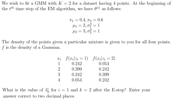
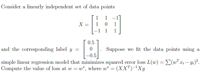
Based on the above data, answer the given subquestions.
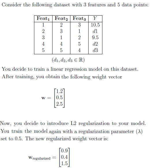
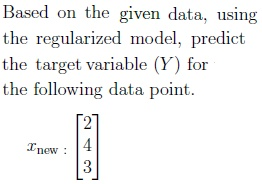
- 7.9
- 12.2
- 11.9
- None of these
If you further reduce the regularization parameter (λ) to zero. What would be the new prediction for the target variable?
- 7.9
- 12.2
- 11.9
- None of these
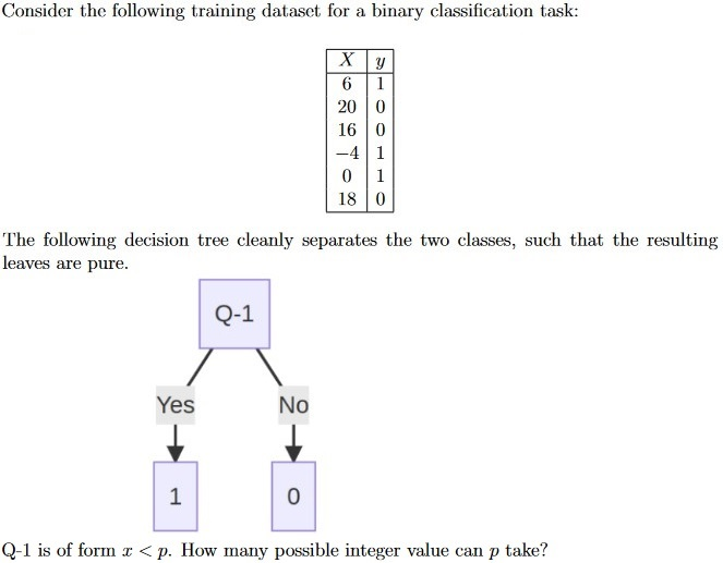

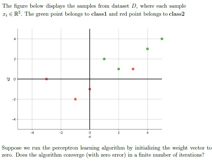
- Yes, it will converge.
- No, it will never converge.
- Insufficient data
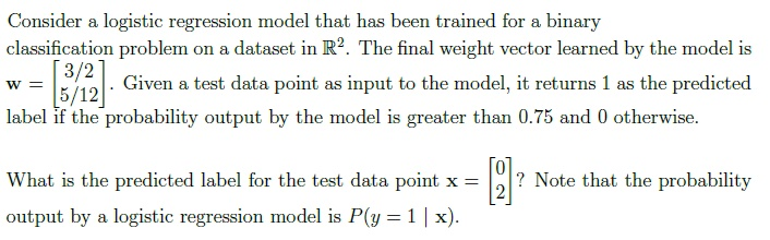
Comprehension passage - the questions below it refer to this
Based on the above data, answer the given subquestions.
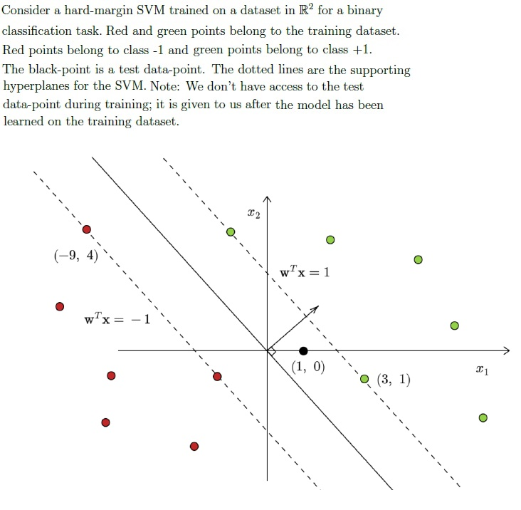
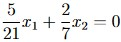
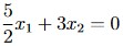
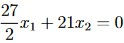
What is the equation of the decision boundary? Select all options that are correct.





Which of the following statements are correct?
- Underfitting models have high bias and low variance.
- Overfitting models have low bias and high variance.
- Generally, weak learners in the random forest tend to underfit.
- If the performance of each estimator in the bagging algorithm is almostidentical, the benefit of using bagging to combine them may be minimal or insignificant.
- In random forests, multiple decision trees (estimators) are trainedsimultaneously, allowing for parallel processing and faster model training.
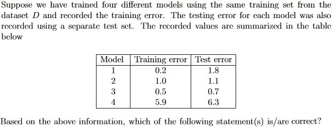
- Model 4 tends to overfit.
- Model 4 tends to underfit.
- Model 1 tends to underfits.
- Model 1 tends to overfits.
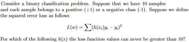
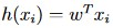


Choose all the correct statements about neural networks
- It can not be used for both regression and classification problems
- It can have more than two hidden layers
- The activation functions have to be non-linear to separate not linearlyseparable data points
- Each neuron in the neural network may or may not have bias associated with it
Answer key
- Q1 (MSQ, 5 marks): A, D
- Q2 (MCQ, 5 marks): D
- Q3 (MSQ, 6 marks): A, B
- Q4 (MSQ, 5 marks): A, C
- Q5 (SA, 6 marks): 0.22 to 0.28
- Q6 (SA, 6 marks): 0
- Q7 (MCQ, 3 marks): A
- Q8 (MCQ, 3 marks): C
- Q9 (SA, 6 marks): 10
- Q10 (SA, 5 marks): 15
- Q11 (MCQ, 5 marks): B
- Q12 (SA, 6 marks): 0
- Q13 (MSQ, 6 marks): A, B, C
- Q14 (SA, 5 marks): 5.32 to 5.44
- Q15 (MSQ, 6 marks): A, B
- Q16 (MSQ, 6 marks): A, B, D, E
- Q17 (MSQ, 5 marks): B, D
- Q18 (MSQ, 5 marks): B, C
- Q19 (MSQ, 6 marks): B, C, D
Concepts this paper tests
Auto-generated summary from the source site. Handy as a checklist; the lessons above explain each idea from scratch.
Here’s a structured summary of core topics, concepts, principles, and equations essential for the exam, followed by Mermaid knowledge graphs to visualize relationships.
Core Topics & Key Concepts
1. Principal Component Analysis (PCA)
- Purpose: Dimensionality reduction while preserving variance.
Steps:
- Center the data (subtract mean).
- Compute covariance matrix: .
- Eigen-decomposition: , where = eigenvectors (principal components), = eigenvalues.
- Project data onto top- eigenvectors.
Key Equations:
- Covariance matrix: .
- Reconstruction error: Zero if (original dimensions).
- First PC: Eigenvector corresponding to the largest eigenvalue.
- Example: For dataset , the first PC is .
2. Linear Regression
- Model: .
- Loss Function (Squared Error): .
- Optimal Weights (Closed-Form): (if is full-rank).
Key Properties:
- Minimum loss at is 0 if data is linearly separable.
- For underdetermined systems, infinite solutions exist.
3. K-Means Clustering
- Algorithm: Lloyd’s algorithm (iterative assignment + centroid update).
Properties:
- Local minima: Depends on initialization (use K-means++ to mitigate).
- Complexity: , where = iterations.
- Choosing : Elbow method or silhouette score.
Trade-offs:
- K-means++ is slower but avoids poor initializations.
- Larger increases computational cost.
4. Decision Trees
Splitting Criteria:
- Gini impurity or entropy for classification.
- Variance reduction for regression.
- Pure Leaves: A leaf is pure if all samples belong to one class.
- Example: For binary classification with threshold in , the number of possible integer values depends on the sorted unique values of .
5. Naive Bayes Classifier
- Assumption: Features are conditionally independent given the class.
Parameters to Learn:
- Class priors: for each class .
- Likelihoods: for each feature , value , and class .
- Example: For 4 classes and 3 binary features, total parameters = (but simplified to 15 if features are binary and symmetries are exploited).
6. Perceptron Algorithm
- Update Rule: if .
- Convergence: Guaranteed if data is linearly separable and learning rate is small.
- Counterexample: Non-separable data (e.g., XOR) leads to no convergence.
7. Logistic Regression
- Model: , where = sigmoid.
- Decision Rule: Predict if (or another threshold).
- Example: For and , compute . If , predict .
8. Support Vector Machines (SVM)
Hard-Margin SVM:
- Optimization: s.t. .
- Decision Boundary: .
- Supporting Hyperplanes: .
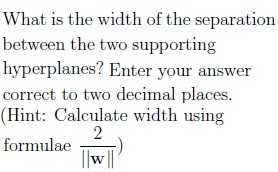
- Margin Width: .
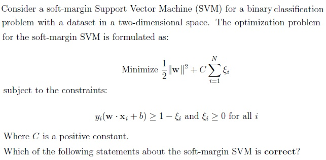
Soft-Margin SVM:
- Allows misclassifications via slack variables .
- Optimization: .
Effect of :
- Small : Wider margin, more misclassifications.
- Large : Narrower margin, fewer misclassifications.
- Kernel Trick: For non-linear boundaries, use (e.g., RBF kernel).
9. Model Evaluation & Bias-Variance Tradeoff
Underfitting:
- High bias, low variance.
- Poor performance on training and test data.
Overfitting:
- Low bias, high variance.
- Good training performance but poor generalization.
Diagnostics:
- Compare training vs. test error (e.g., Model 1 in Q18 overfits; Model 4 underfits).
10. Ensemble Methods (Bagging & Random Forest)
Bagging:
- Train multiple models on bootstrapped samples.
- Average predictions (regression) or vote (classification).
- Reduces variance.
Random Forest:
- Extension of bagging with feature randomness.
- Parallelizable (trees are independent).
- Weak learners (shallow trees) are preferred to avoid overfitting.
11. Neural Networks
Architecture:
- Input layer, hidden layers (with non-linear activations), output layer.
Key Properties:
- Universal approximator with sufficient hidden units.
- Non-linear activations (e.g., ReLU, sigmoid) are essential for non-linear decision boundaries.
- Bias terms are optional but typically included.
12. Regularization
L1/L2 Regularization:
- Add (Lasso) or (Ridge) to loss.
Effect of :
- : Approaches unregularized solution.
- : Weights .
Key Equations Summary
| Topic | Equation |
|---|---|
| PCA Covariance | |
| Linear Regression | |
| Logistic Regression | |
| SVM Hard Margin | s.t. |
| SVM Margin Width | |
| Perceptron Update | if misclassified |
| MSE Loss | |
| Soft-Margin SVM |
Graph 2: Classification Algorithms
Graph 3: Model Evaluation & Ensemble Methods
Graph 4: Optimization & Regularization
Exam Tips
- PCA: Always center the data first. The first PC is the eigenvector with the largest eigenvalue.
- SVM: The margin width is . Supporting hyperplanes are .
- Logistic Regression: Predict class based on vs. threshold (default 0.5).
- Decision Trees: Count unique splits for pure leaves.
- Naive Bayes: Parameters = (classes) × (features) × (feature values) + (class priors).
- Perceptron: Only converges if data is linearly separable.
- Regularization: removes regularization; forces weights to zero.