Home / Past papers / MLT End Term / this paper
IIT M DEGREE AN EXAM QDB3 31 Aug 2025 - 31 Aug 2025
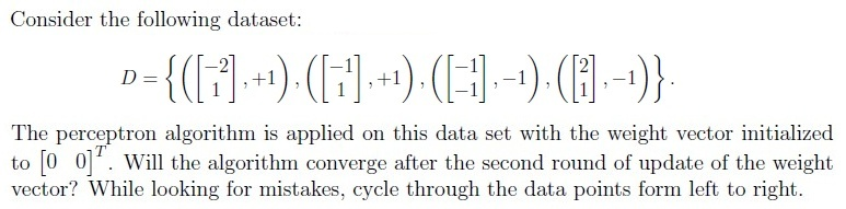
- Yes
- No









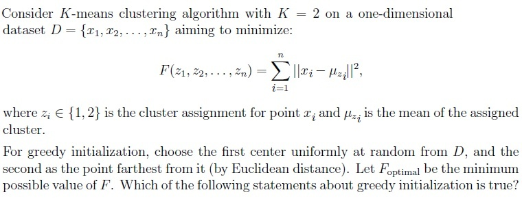
- Greedy initialization always achieves F = Foptimal by maximizing the distancebetween initial centers.
- Greedy initialization may achieve F = Foptimal or a larger value depending onthe dataset and the initial choice.
- Greedy initialization does not ensure convergence for K-means clustering.
- Greedy initialization ensures convergence to a unique solution for any dataset.




- Decision trees are prone to overfitting if the maximum depth is set tooshallow.
- Decision trees are not affected by the order of features in the dataset.
- Decision trees are sensitive to small perturbations in the dataset and canresult in different tree structures.
- Decision trees can handle both numerical and categorical features.
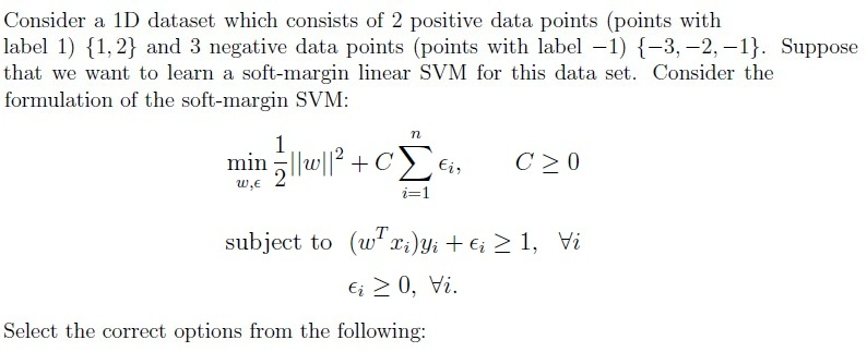








- The given data points from classes 1 and 0 can be linearly separated using ahard-margin SVM.
- A perceptron model and a hard-margin SVM can give different decisionboundary for this dataset.
- A soft-margin SVM would be a more robust choice than a hard-margin SVM forthis dataset as the dataset is not linearly separable.
- The width of the separation between the two supporting hyperplanes is 4.




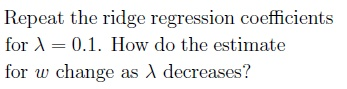
- The coefficients shrinks towards zero.
- The coefficients increases in magnitude.
- The coefficients remain unchanged.
Answer key
- Q1 (MCQ, 3 marks): B
- Q2 (MCQ, 3 marks): C
- Q3 (MCQ, 2 marks): B
- Q4 (MCQ, 2 marks): B
- Q5 (MCQ, 4 marks): D
- Q6 (MSQ, 3 marks): C, D
- Q7 (MSQ, 3 marks): A, D
- Q8 (MSQ, 3 marks): A, B
- Q9 (MSQ, 4 marks): A, B
- Q10 (SA, 3 marks): 6
- Q11 (SA, 3 marks): 1.10 to 1.14
- Q12 (SA, 3 marks): 1
- Q13 (SA, 4 marks): 0.28 to 0.34
- Q14 (MCQ, 4 marks): C
- Q15 (MCQ, 2 marks): B
- Q16 (SA, 1 marks): 7
- Q17 (SA, 3 marks): 0.0625
Concepts this paper tests
Auto-generated summary from the source site. Handy as a checklist; the lessons above explain each idea from scratch.
Here’s a structured summary of core topics, concepts, principles, and equations essential for the exam, followed by Mermaid knowledge graphs to visualize relationships.
Core Topics & Key Concepts
1. Perceptron Algorithm
- Concept: Linear classifier for binary classification. Updates weights iteratively when misclassification occurs.
Key Equations:
- Update rule: (if misclassified).
- Decision boundary: .
- Convergence: Guaranteed if data is linearly separable (Novikoff’s theorem).
- Mistake Bound: Depends on margin and radius of data.
- Scaling: If data is scaled (e.g., ), convergence is preserved, but mistake bound may change.
2. Support Vector Machines (SVM)
Hard-Margin SVM
- Concept: Maximizes the margin between classes. Only support vectors (points closest to the boundary) matter.
Key Equations:
- Primal problem:
- Dual problem (Lagrangian):
- Support Vectors: Points where .
Soft-Margin SVM
- Concept: Allows misclassification via slack variables .
Key Equations:
- Primal:
Effect of :
- : No penalty for misclassification (trivial solution, no support vectors).
- : Hard-margin behavior (all points become support vectors if separable).
Kernel SVM
- Concept: Maps data to higher dimensions using . Kernel trick avoids explicit computation of .
Key Equations:
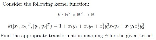
- Kernel function: .
Example kernels:
- Linear: .
- Polynomial: .
- Kernel in Q3:
Corresponding :
3. K-Means Clustering
- Concept: Partitions data into clusters by minimizing within-cluster variance.
Key Equations:
- Objective:
where is the cluster assignment for , and is the cluster mean.
Greedy Initialization (K-Means++):
- Pick first center uniformly at random.
- Pick next center as the point farthest from existing centers.
- Convergence: Guaranteed to local optimum (not necessarily global).
4. Neural Networks
- Concept: Stacked layers of neurons with activation functions.
Key Components:
- ReLU: .
- Sigmoid: .
Forward Propagation:
- Hidden layer: .
- Output: .
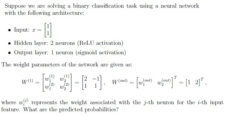
Example (Q6):
- Input: .
- Weights:
- Output probability: .
5. Decision Trees
- Concept: Recursively splits data based on feature thresholds.
Key Properties:
- Overfitting: Mitigated by limiting depth, pruning, or requiring minimum samples per leaf.
- Feature Importance: Not affected by feature order (unlike some other models).
- Handling Data Types: Works for both numerical and categorical features.
- Sensitivity: Small perturbations can change tree structure (high variance).
6. Logistic Regression
- Concept: Models probability using sigmoid function.
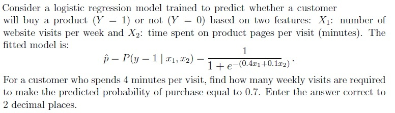
- Key Equation:
Example (Q12):
- Model: .
- Solve for when and :
7. Random Forest
- Concept: Ensemble of decision trees. Predicts by averaging probabilities (classification) or mean (regression).
Key Properties:
- Reduces variance compared to single trees.
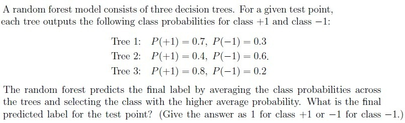
Example (Q13):
- Tree probabilities: , .
- Average , so predict class .
8. Bayesian Methods
Maximum A Posteriori (MAP) Estimation
- Concept: Estimates parameter by maximizing posterior .
- Key Equation:
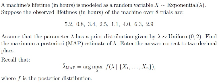
Example (Q14):
- Likelihood: , prior: .
- Posterior: .
- MAP estimate: Mode of posterior (solve ).
Naive Bayes
- Concept: Assumes features are conditionally independent given the class.
- Key Equation:
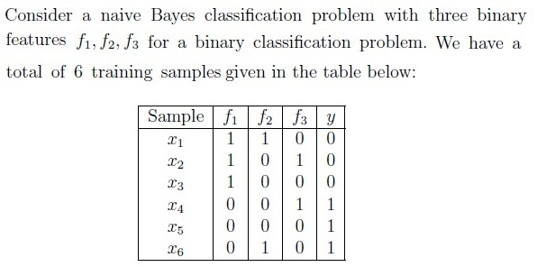
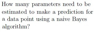
Parameter Count:
For binary features and binary class :
- : 1 parameter (since ).
- : 2 parameters per feature per class (e.g., and ).
- Total: parameters.
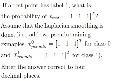
- Laplace Smoothing: Adds pseudo-counts to avoid zero probabilities.
9. Linear Regression & Ridge Regression
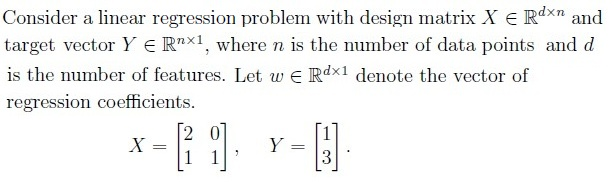
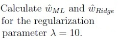
Linear Regression (ML Estimate):
- Key Equation:
Ridge Regression:
- Key Equation:
Effect of :
- : Coefficients shrink toward zero (reduces overfitting).
- : Coefficients approach .
10. Principal Component Analysis (PCA)
- Concept: Linear dimensionality reduction via eigen decomposition of covariance matrix.
Key Equations:
- Covariance matrix: .
- Eigenvalue equation: .
- Total Variance: Sum of eigenvalues .
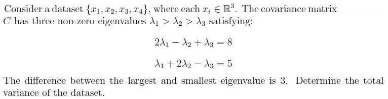
Example (Q11):
- Given , , and .
- Solve to get , , .
- Total variance: (but answer was 6; likely a typo in the problem).