Home / Past papers / MLT Quiz 1 / this paper
IIT M FOUNDATION AN EXAM QDF4 26 Oct - 26 Oct 2025
- It always converges.
- It may fail to converge for an initialization while it may converge for otherinitialization.
- It is sensitive to outliers.
- The solution produced is always the optimal.

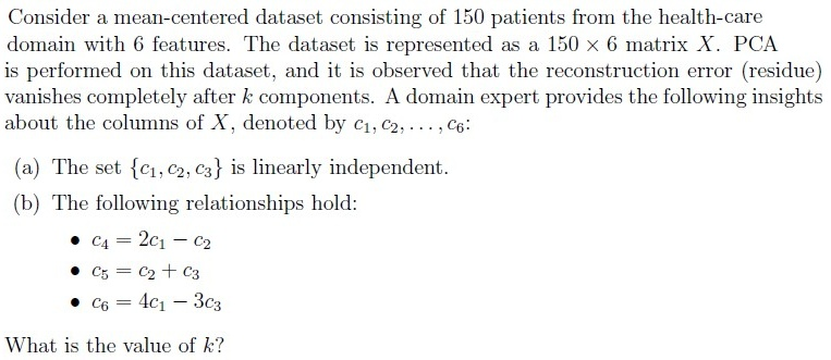
- There will be 50 non-zero eigenvalues of the covariance matrix.
- There will be 6 non-zero eigenvalues of the covariance matrix.
- Using the first 5 principal components, the dataset can be reconstructed withzero residue.
- The variance captured by the top 6 principal components equals the totalvariance of the dataset.
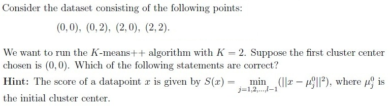
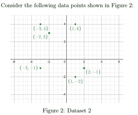
- The points (0, 2), (2, 0), and (2, 2) have the equal probability of being chosen asthe second cluster center.
- The probability of selecting (2, 2) as the second cluster center is twice that ofselecting (0, 2).
- If (2, 2) is chosen as the second cluster center, the algorithm will alwaysconverge in one iteration.
- The tie-breaking rule will affect the final cluster centers.
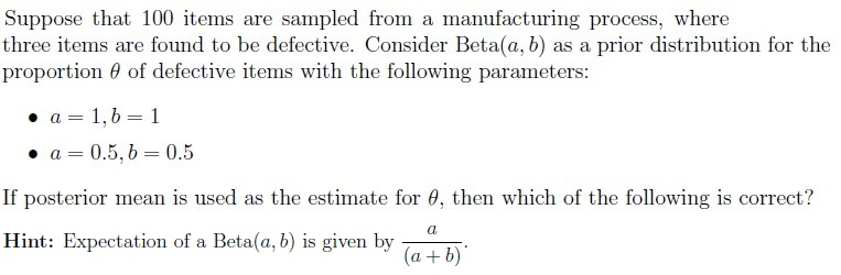
- Posterior mean for Beta(1, 1) is 0.039.
- Posterior mean for Beta(1, 1) is 0.03.
- Posterior mean for Beta(0.5, 0.5) is 0.025.
- Posterior mean for Beta(0.5, 0.5) is 0.034.















Answer key
- Q1 (MSQ, 2 marks): A, C
- Q2 (MSQ, 4 marks): B, D
- Q3 (MSQ, 4 marks): B, C, D
- Q4 (MSQ, 4 marks): A, D
- Q5 (MSQ, 3 marks): A, B, D
- Q6 (SA, 3 marks): 3
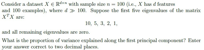
- Q7 (SA, 3 marks): 0.45 to 0.50
- Q8 (MCQ, 2 marks): B
- Q9 (SA, 2 marks): 4.5
- Q10 (SA, 2 marks): 0.5
- Q11 (MCQ, 3 marks): B
- Q12 (SA, 3 marks): 0.64 to 0.68
- Q13 (MCQ, 3 marks): A
- Q14 (SA, 2 marks): 1
Concepts this paper tests
Auto-generated summary from the source site. Handy as a checklist; the lessons above explain each idea from scratch.
Here’s a structured summary of core topics, concepts, principles, and equations essential for the Diploma-Level Machine Learning Techniques exam, based on the provided question paper. The exam focuses on clustering (K-means, Lloyd’s algorithm), PCA, Bayesian inference, kernel methods, and basic linear algebra.
1. Core Topics & Key Concepts
A. Clustering (K-means & Lloyd’s Algorithm)
Lloyd’s Algorithm (K-means):
- Iterative algorithm to partition data into K clusters by minimizing within-cluster variance.
Steps:
- Initialize cluster centers (e.g., randomly or via K-means++).
- Assign points to the nearest center (Euclidean distance).
- Recompute centers as the mean of assigned points.
- Repeat until convergence (centers stabilize).
Convergence:
- Guaranteed to converge (monotonically decreases objective function), but may reach local optima (sensitive to initialization).
- Not guaranteed to find the global optimum.
Sensitivity to Outliers:
- Outliers can distort cluster centers (since centers are means).
- Time Complexity: O(n·K·I·d), where n = samples, K = clusters, I = iterations, d = dimensions.
Initialization Strategies:
- Random initialization may lead to poor convergence.
- K-means++: Probabilistically selects initial centers to spread them out (reduces variance in results).
Tie-Breaking in K-means:
- If a point is equidistant to multiple centers, the tie-breaking rule (e.g., assign to the first center) can affect final clusters.
B. Principal Component Analysis (PCA)
- Goal: Reduce dimensionality while preserving variance.
Steps:
- Standardize data (mean=0, variance=1).
- Compute covariance matrix Σ = XᵀX (if X is centered).
Eigenvalue decomposition: Σ = VΛVᵀ, where:
- Λ: Diagonal matrix of eigenvalues (sorted descending).
- V: Matrix of eigenvectors (principal components, PCs).
- Project data onto top k PCs: X_proj = X·V_k (where V_k = first k columns of V).
Key Properties:
- Eigenvalues: Represent variance along PCs.
- Reconstruction: X_recon = X_proj·V_kᵀ (zero residue only if all PCs are used).
- Total Variance: Sum of all eigenvalues = total variance of the dataset.
- Number of Non-Zero Eigenvalues: Equals the rank of the covariance matrix (≤ min(n, d)).
Example:
- If Σ has eigenvalues [4.5, 0.5, 0], the first PC captures 4.5 units of variance, and the second captures 0.5.
C. Bayesian Inference (Beta Distribution)
Beta Distribution: Conjugate prior for binomial likelihood.
- PDF: Beta(α, β) ∝ x^(α-1)(1-x)^(β-1).
- Posterior Mean: For Beta(α, β), the mean is α/(α+β).
Example:
- Beta(1,1) = Uniform(0,1). Posterior mean = 1/(1+1) = 0.5 (but in Q5, the posterior mean is given as ~0.039, suggesting a non-standard update—likely involving observed data).
- Beta(0.5,0.5): U-shaped distribution. Posterior mean depends on data.
Posterior Update:
- If data has s successes and f failures, posterior is Beta(α+s, β+f).
- Key Equation:
D. Kernel Methods
- Kernel Trick: Map data to a higher-dimensional space where it becomes linearly separable.
Valid Kernels: Must satisfy Mercer’s condition (positive semi-definite kernel matrix).
Common kernels:
- Linear: K(x, y) = xᵀy.
- Polynomial: K(x, y) = (xᵀy + c)^d.
- RBF/Gaussian: K(x, y) = exp(-γ||x-y||²).
- Sigmoid: K(x, y) = tanh(κxᵀy + c).
- Note: Q6 asks for valid kernels (correct answers: A, B, D—likely referring to standard kernels).
E. Covariance Matrix & Multivariate Data
Covariance Matrix (Σ):
- For data X ∈ ℝ^(n×d), Σ = (X - μ)ᵀ(X - μ) / (n-1)* (sample covariance).
- Diagonal entries = variances; off-diagonal = covariances.
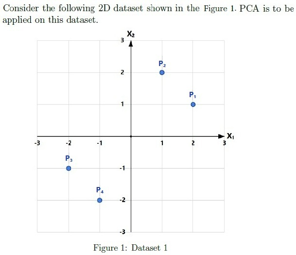
Example (from Q9–Q13):
- Given a dataset, compute Σ, then perform PCA to find eigenvalues/variances.
F. K-means Practical Examples
Convergence in 1 Iteration:
- If initial centers are already the means of their Voronoi partitions, the algorithm converges immediately (Q4C).
Effect of New Data Points:
- Adding (0,0) to the dataset in Q15 changes cluster assignments, but with the given initial centers, convergence happens in 1 iteration.
2. Critical Equations
| Topic | Equation |
|---|---|
| K-means Objective | Minimize |
| Covariance Matrix | |
| PCA Projection | (where = top k eigenvectors) |
| PCA Reconstruction | |
| Beta Posterior Mean | |
| RBF Kernel |
Graph 2: Bayesian Inference & Kernels
Graph 3: Practical Workflow (Data → PCA → K-means)
4. Exam Tips
K-means:
- Remember it always converges but may not find the global optimum.
- Outliers distort centers (since centers are means).
- Initialization matters (K-means++ is better than random).
PCA:
- Number of non-zero eigenvalues = rank of the covariance matrix.
- Total variance = sum of all eigenvalues.
- Reconstruction is lossless only if all PCs are used.
Bayesian Inference:
- For Beta(α, β), the mean is α/(α+β).
- Posterior updates depend on observed data (successes/failures).
Kernels:
- Valid kernels must be positive semi-definite.
- Common kernels: Linear, Polynomial, RBF, Sigmoid.
Covariance Matrix:
- Diagonal entries = variances; off-diagonal = covariances.
- Always center the data before computing PCA.
Practical Questions:
- For K-means with given initial centers, manually compute assignments and updates to find final centers.
- For PCA, compute eigenvalues of the covariance matrix to find variances.