Home / Past papers / MLT End Term / this paper

IIT M DIPLOMA ET1 EXAM QPD1 S1 03 Sep - 03 Sep 2023

MLT End Term17 questions100 marks8 MSQ · 5 SA · 4 MCQDiploma / QPD1

Elapsed 00:00

Q1SA6 marks

Your numeric answer:

Q2SA6 marks

Your numeric answer:

Q3SA6 marks

Hint: Assume that these are only two possible words (that is there are only two features) question figure

Your numeric answer:

Q4MSQ6 marksselect all that apply

Q5MSQ6 marksselect all that apply

Q6MSQ6 marksselect all that apply

Which of the following statements is/are true?

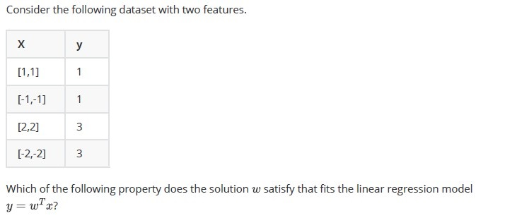
Ridge regression and Lasso regression both puts a limit on the length ofweight vector.
Ridge regression puts limit on length of the weight vector but LASSOregression does not put a limit on weight vector length.
When many features are redundant, then LASSO regression is moreappropriate than ridge regression and linear regression as LASSO regression produces sparseweights for those features.
When many features are redundant, then linear regression is moreappropriate than ridge regression and LASSO regression

Q7MSQ6 marksselect all that apply

Q8MSQ6 marksselect all that apply

Q9MSQ6 marksselect all that apply

Q10MCQ6 marks

Q11MCQ6 marks

Q12MCQ6 marks

Q13MCQ6 marks

Q14SA5 marks

Your numeric answer:

Q15MSQ3 marksselect all that apply

Which of the following statements is/are true about the K-NN algorithm?

K-NN is sensitive to outliers in the dataset.
K-NN is a supervised learning algorithm used for classification.
K-NN assigns class labels to new instances based on a decision boundary learned from thetraining data.
The training dataset is not required while predicting the label of a test-point inthe K-NN algorithm.

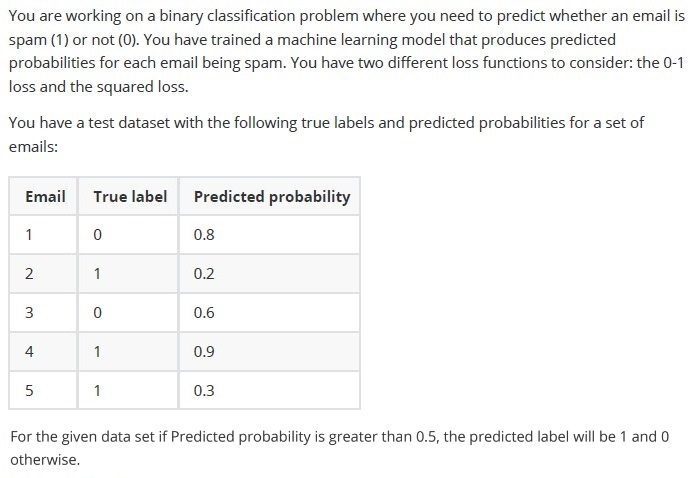
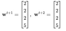
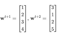
Q16MSQ7 marksselect all that apply

The values of 0-1 loss function will be 3
The values of squared loss will be equals to 2.14
The values of 0-1 loss equals 4.
The values of squared loss will be equals to 3.14

Q17SA7 marks

Your numeric answer:

Answer key

Q1 (SA, 6 marks): 34
Q2 (SA, 6 marks): 0.120 to 0.180
Q3 (SA, 6 marks): 0.98 to 1
Q4 (MSQ, 6 marks): A, B
Q5 (MSQ, 6 marks): A, C, D
Q6 (MSQ, 6 marks): A, C
Q7 (MSQ, 6 marks): B, D
Q8 (MSQ, 6 marks): B, C
Q9 (MSQ, 6 marks): B, C, D
Q10 (MCQ, 6 marks): A
Q11 (MCQ, 6 marks): A
Q12 (MCQ, 6 marks): D
Q13 (MCQ, 6 marks): D
Q14 (SA, 5 marks): 0.10 to 0.60
Q15 (MSQ, 3 marks): A, B
Q16 (MSQ, 7 marks): B, C
Q17 (SA, 7 marks): 0.60 to 0.80

Concepts this paper tests

Auto-generated summary from the source site. Handy as a checklist; the lessons above explain each idea from scratch.

Here’s a structured summary of core topics, concepts, principles, and equations for the Diploma-Level Machine Learning Techniques exam, along with Mermaid knowledge graphs to visualize relationships.

1. Core Topics & Key Concepts

A. Dimensionality Reduction (PCA)

Purpose: Reduce feature space while preserving variance.
Steps:
1. Center the data (subtract mean).
2. Compute covariance matrix $\Sigma = \frac{1}{n} X^T X$ .
3. Eigen-decomposition: $\Sigma = V \Lambda V^T$ , where:
  - $\Lambda$ : Diagonal matrix of eigenvalues $\lambda_1 \geq \lambda_2 \geq ... \geq \lambda_d$ .
  - $V$ : Matrix of eigenvectors (principal components).
4. Project data: $X_{\text{PCA}} = X V_k$ (top- $k$ eigenvectors).
Total Variance: Sum of eigenvalues.
- Equation: $\text{Variance} = \sum_{i=1}^d \lambda_i$ .
Explained Variance Ratio: $\frac{\lambda_i}{\sum \lambda_j}$ .

Key Equation:

\text{Variance} = \lambda_1 + \lambda_2 + ... + \lambda_d

B. Bayesian Estimation

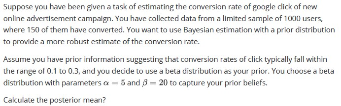
Prior: Beta distribution $\text{Beta}(\alpha, \beta)$ .
Likelihood: Binomial distribution (for binary outcomes).
Posterior: Updated Beta distribution.
- Posterior Parameters:

\alpha' = \alpha + \text{successes}, \quad \beta' = \beta + \text{failures}

Posterior Mean:

\text{Mean} = \frac{\alpha'}{\alpha' + \beta'}

Key Equation:

P(\theta | \text{data}) = \text{Beta}(\alpha + \text{successes}, \beta + \text{failures})

C. Naive Bayes Classifier

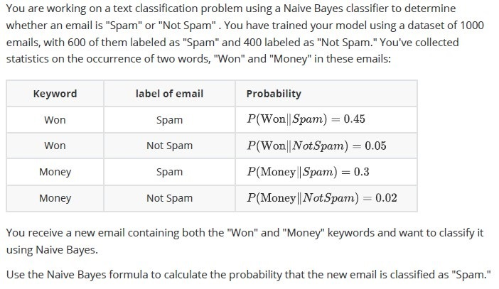
Assumption: Features are conditionally independent given the class.
Posterior Probability:

P(y | x_1, ..., x_n) \propto P(y) \prod_{i=1}^n P(x_i | y)

Prediction: Choose class with highest posterior.

Key Equation:

\hat{y} = \argmax_y P(y) \prod_{i=1}^n P(x_i | y)

D. Gram Matrix & Kernel Methods

Gram Matrix: $K = X^T X$ (symmetric and positive semi-definite).
Properties:
- Symmetry: $K = K^T$ .
- Positive Semi-Definite: $v^T K v \geq 0$ for any $v$ .

Key Check: For a matrix $K$ to be a Gram matrix:

$K = K^T$ .
All eigenvalues $\geq 0$ .

E. Clustering (Lloyd’s Algorithm / K-Means)

Objective: Minimize within-cluster sum of squares (WCSS).
Steps:
1. Initialize centroids.
2. Assign points to nearest centroid.
3. Update centroids as mean of assigned points.
4. Repeat until convergence.
Decision Boundary: Voronoi diagram (points assigned to nearest centroid).

Key Insight: Points closer to existing cluster centroids (e.g., $[0, 0]^T$ ) are likely in the same cluster.

F. Regularization (Ridge vs. Lasso)

Aspect	Ridge (L2)	Lasso (L1)
Penalty	$\lambda \sum w_j^2$	$\lambda \sum \|w_j\|$
Effect	Shrinks weights	Shrinks + sets weights to 0 (sparse)
Use Case	Multicollinearity	Feature selection

Key Equations:

\text{Ridge: } \min \|y - Xw\|_2^2 + \lambda \|w\|_2^2

\text{Lasso: } \min \|y - Xw\|_2^2 + \lambda \|w\|_1

G. Support Vector Machines (SVM)

Hard Margin SVM: Maximize margin $\frac{2}{\|w\|}$ with no misclassifications.
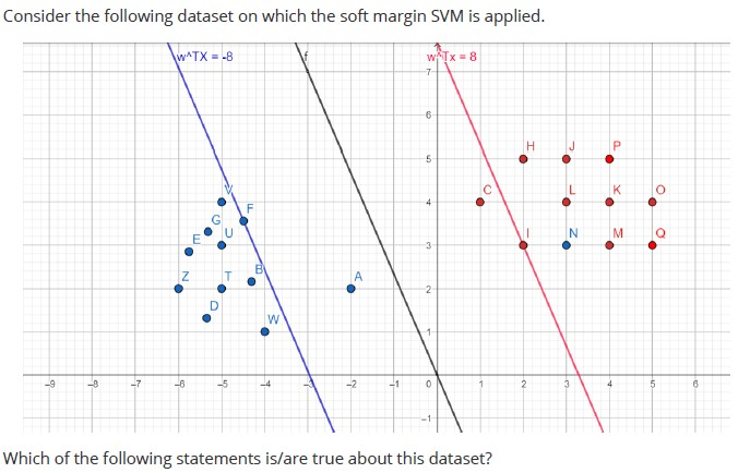
Soft Margin SVM: Allow misclassifications (slack variables $\xi_i$ ).
- Primal Problem:

\min_{w, b, \xi} \frac{1}{2} \|w\|^2 + C \sum \xi_i \quad \text{s.t.} \quad y_i (w^T x_i + b) \geq 1 - \xi_i, \xi_i \geq 0

Dual Problem:

\max_\alpha \sum \alpha_i - \frac{1}{2} \sum_{i,j} \alpha_i \alpha_j y_i y_j x_i^T x_j \quad \text{s.t.} \quad 0 \leq \alpha_i \leq C, \sum \alpha_i y_i = 0

Support Vectors: Points with $\alpha_i > 0$ .
Kernel Trick: Replace $x_i^T x_j$ with $K(x_i, x_j)$ .

Key Insights:

If $\alpha_i^* = 0$ :
- Point is correctly classified with margin $> 1$ .
- No slack ( $\xi_i = 0$ ).
If $0 < \alpha_i^* < C$ :
- Point is a support vector on the margin.
If $\alpha_i^* = C$ :
- Point is misclassified or within the margin.

H. Random Forest

Bagging: Bootstrap aggregating (reduce variance).
Feature Subsampling: At each split, randomly select $p$ features from $d$ total.
- Effect of $p$ :
  - Small $p$ : Decorrelates trees (reduces variance) but may underfit.
  - Large $p$ : Trees become similar (increases variance).
Out-of-Bag (OOB) Error: Estimate generalization error without a separate validation set.

Key Trade-offs: | $p$ (Features) | Correlation | Bias | Variance | |------------------------|----------------|----------|--------------| | Small | Low | High | Low | | Large | High | Low | High |

I. Linear Regression

Model: $y = w^T x + \epsilon$ .
Ordinary Least Squares (OLS):

w = (X^T X)^{-1} X^T y

Assumptions:
- Linear relationship.
- No multicollinearity.
- Homoscedasticity (constant variance of errors).

Key Equation:

w = \argmin_w \|y - Xw\|_2^2

J. Perceptron Algorithm

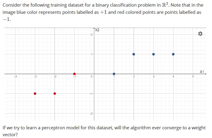
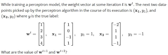
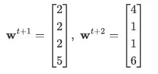
Update Rule: If $y_i (w^T x_i + b) \leq 0$ , update:

w \leftarrow w + \eta y_i x_i, \quad b \leftarrow b + \eta y_i

Convergence: Guaranteed if data is linearly separable.

Key Insight:

If $y_i (w^T x_i + b) > 0$ , no update is needed.

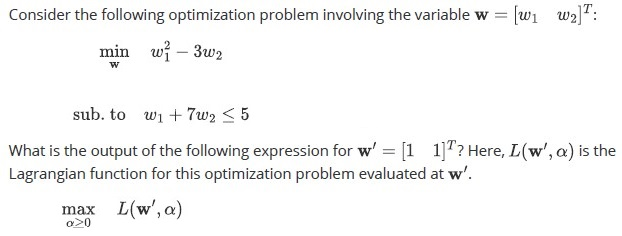
K. Optimization (Lagrangian)

Primal Problem: $\min_w f(w)$ s.t. $g(w) \leq 0$ .
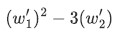
Lagrangian:

L(w, \alpha) = f(w) + \alpha g(w)

Dual Problem: $\max_{\alpha \geq 0} \min_w L(w, \alpha)$ .

Key Equation:

\max_{\alpha \geq 0} L(w', \alpha) = \begin{cases} f(w') & \text{if } g(w') \leq 0 \\ \infty & \text{otherwise} \end{cases}

L. Decision Trees

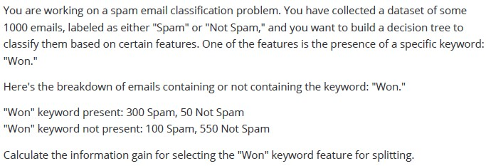
Information Gain (IG):

IG = H(\text{parent}) - \sum \frac{N_j}{N} H(\text{child}_j)

where $H$ is entropy:

H(S) = - \sum p_i \log_2 p_i

Splitting Criterion: Maximize IG.

Key Equation:

IG(\text{feature}) = H(\text{target}) - H(\text{target} | \text{feature})

M. K-Nearest Neighbors (K-NN)

Prediction: Majority vote (classification) or average (regression) of $k$ nearest neighbors.
Distance Metric: Typically Euclidean or Manhattan.
Sensitivity:
- Outliers: High $k$ reduces impact.
- Scale: Features should be normalized.

Key Insight:

Lazy learner (no training phase).
Computationally expensive at test time.

N. Loss Functions

Loss Function	Equation	Use Case
0-1 Loss	$\mathbb{I}(y \neq \hat{y})$	Classification accuracy
Squared Loss	$(y - \hat{y})^2$	Regression (e.g., MSE)
Cross-Entropy	$-\sum y_i \log \hat{y}_i$	Probabilistic classification

Key Equations:

\text{0-1 Loss} = \sum_{i=1}^n \mathbb{I}(y_i \neq \hat{y}_i)

\text{Squared Loss} = \sum_{i=1}^n (y_i - \hat{y}_i)^2

O. Neural Networks

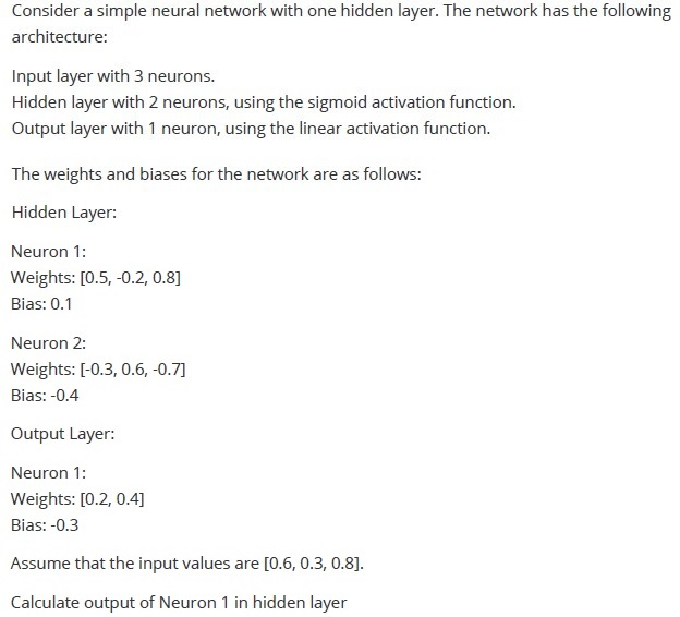
Forward Propagation:

z^{(l)} = W^{(l)} a^{(l-1)} + b^{(l)}, \quad a^{(l)} = \sigma(z^{(l)})

where $\sigma$ is the activation function (e.g., sigmoid, ReLU).

Sigmoid:

\sigma(z) = \frac{1}{1 + e^{-z}}

Key Equation:

a^{(l)} = \sigma(W^{(l)} a^{(l-1)} + b^{(l)})

Graph 2: Dimensionality Reduction & Clustering

Graph 3: Optimization & Model Training

Graph 4: Bayesian vs. Frequentist

Graph 5: Ensemble Methods

3. Key Equations Summary

Topic	Equation
PCA Variance	$\text{Variance} = \sum_{i=1}^d \lambda_i$
Bayesian Posterior	$\alpha' = \alpha + \text{successes}, \beta' = \beta + \text{failures}$
Naive Bayes	$\hat{y} = \argmax_y P(y) \prod P(x_i \| y)$
SVM Primal	$\min \frac{1}{2} \\|w\\|^2 + C \sum \xi_i$
SVM Dual	$\max_\alpha \sum \alpha_i - \frac{1}{2} \sum \alpha_i \alpha_j y_i y_j x_i^T x_j$
Information Gain	$IG = H(S) - \sum \frac{\|S_v\|}{\|S\|} H(S_v)$
Perceptron Update	$w \leftarrow w + \eta y_i x_i$ if misclassified
Lagrangian	$L(w, \alpha) = f(w) + \alpha g(w)$
Linear Regression	$w = (X^T X)^{-1} X^T y$
Ridge/Lasso	$\min \\|y - Xw\\|_2^2 + \lambda \\|w\\|_{1/2}^2$
0-1 Loss	$\sum \mathbb{I}(y_i \neq \hat{y}_i)$
Squared Loss	$\sum (y_i - \hat{y}_i)^2$
Sigmoid	$\sigma(z) = \frac{1}{1 + e^{-z}}$

4. Exam Tips

PCA: Always check eigenvalues for variance and eigenvectors for principal components.
Bayesian: Remember to add successes/failures to $\alpha/\beta$ .
Naive Bayes: Multiply conditional probabilities (assume independence).
SVM: $\alpha_i = 0$ implies correct classification outside margin.
Random Forest: Lower $p$ reduces correlation but may underfit.
Perceptron: Only update weights if misclassified.
Decision Trees: Calculate entropy and information gain for splits.
K-NN: Normalize features and choose $k$ carefully (odd for binary classification).
Loss Functions: 0-1 loss counts misclassifications; squared loss penalizes large errors.
Neural Networks: Forward propagation is layer-by-layer activation.