Home / Past papers / MLT End Term / this paper
IIT M DIPLOMA FN EXAM QDD2 13 Apr 2025 - 13 Apr 2025
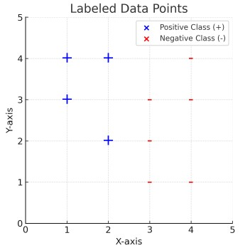 For a given dataset, a 1-Nearest Neighbor (1-NN) and a 3-Nearest Neighbor (3-NN) classifier are applied. Which classifier is likely to exhibit a higher Leave-One-Out Cross Validation (LOOCV) error? In case of tie-breaker, assign a positive class (+) to the data point.
- 1-NN
- 3-NN
- Both have the same error.





- PCA maximizes variance in the original feature space, while Kernel PCAmaximizes variance in a higher-dimensional transformed space.
- PCA finds principal components using linear transformations in the originalspace, while Kernel PCA uses non-linear transformations to find principal components in a higher-dimensional space.
- Kernel PCA can capture non-linear patterns in data, making it useful when PCAfails to represent complex structures in a linear space.
- PCA and Kernel PCA always yield identical results regardless of the datasetstructure.





- The final model has lesser variance than the individual learners.
- The final model has a higher variance than the individual learners.
- Estimators in bagging can be trained parallely.
- If the number of data points is large, typically two-third of the data pointsremain unselected in bags.

- It penalizes large coefficients to reduce overfitting.
- It shrinks the coefficients but does not set them to zero.
- It forces more coefficients to be exactly zero, performing feature selection.
- It has no effect on the regression model.
- YES
- NO
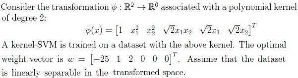

- It is a circle.
- It is a straight line.
- It is an ellipse.
- It is a parabola.


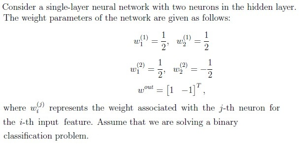
Answer key
- Q1 (MCQ, 3 marks): A
- Q2 (MCQ, 3 marks): C
- Q3 (MCQ, 4 marks): B
- Q4 (MCQ, 4 marks): B
- Q5 (MSQ, 3 marks): A, B, C
- Q6 (MSQ, 3 marks): B, D, E
- Q7 (MSQ, 2 marks): A, C
- Q8 (MSQ, 2 marks): A, C
- Q9 (SA, 2 marks): 8
- Q10 (SA, 3 marks): 24
- Q11 (SA, 3 marks): 20
- Q12 (SA, 3 marks): 11
- Q13 (SA, 3 marks): 1
- Q14 (MCQ, 2 marks): A
- Q15 (MCQ, 2 marks): C
- Q16 (MSQ, 3 marks): A, C
- Q17 (SA, 3 marks): 0.64 to 0.68
- Q18 (SA, 2 marks): 1
Concepts this paper tests
Auto-generated summary from the source site. Handy as a checklist; the lessons above explain each idea from scratch.
Here’s a structured summary of core topics, concepts, principles, and equations for the Diploma-Level Machine Learning Techniques exam, along with Mermaid knowledge graphs to visualize relationships.
1. Core Topics & Key Concepts
A. Supervised Learning
k-Nearest Neighbors (k-NN)
- LOOCV Error: 1-NN often has higher variance (overfits) than 3-NN, leading to higher LOOCV error.
- Tie-Breaker: Assign positive class (
+) if ties occur. - Key Idea: Larger
ksmooths decision boundaries (reduces overfitting).
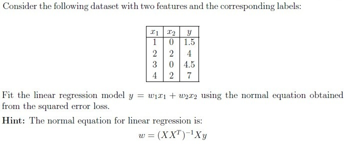
Linear Regression (Normal Equation)
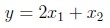
- Model:
- Normal Equation:
- Assumptions: Linear relationship, no multicollinearity, homoscedasticity.
Ridge Regression (L2 Regularization)
- Objective:
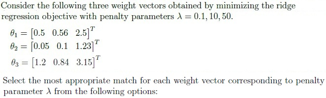
Effect of λ:
- High λ: Shrinks coefficients toward zero (underfitting).
- Low λ: Coefficients approach OLS solution (overfitting).
- Example: Match vectors to values (smaller → larger ).
Lasso Regression (L1 Regularization)
- Objective:
Effect of λ:
- Increases λ: Forces more coefficients to exactly zero (feature selection).
- Sparsity: Unlike Ridge, Lasso performs automatic feature selection.
Support Vector Machines (SVM)
- Hard-Margin SVM:
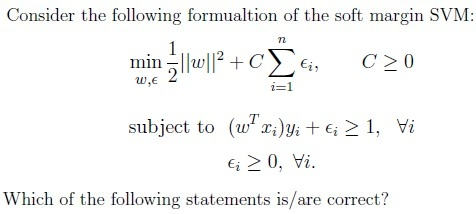
- Soft-Margin SVM:
Effect of C:
- C → 0: Approaches hard-margin (no slack).
- C → ∞: Allows more slack (overfitting).
- Kernel Trick: Transforms data to higher dimensions (e.g., polynomial kernel → ellipse decision boundary).
AdaBoost
- Weight Update: Misclassified points get higher weights in next iteration.
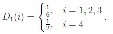
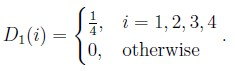
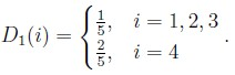
- Example: If 1 point is misclassified (out of 4), its weight increases to 1/2, others decrease to 1/6.
- Formula:
where .
Decision Trees
- Binary Tree: Each node splits into 2 children.
- Leaf Nodes: For depth
d, number of leaves = . - Example: Depth 3 → 8 leaves.
B. Unsupervised Learning
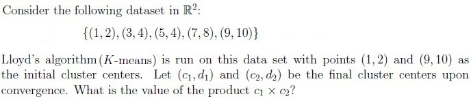
K-Means (Lloyd’s Algorithm)
Steps:
- Initialize centroids (e.g., and ).
- Assign points to nearest centroid.
- Update centroids as mean of assigned points.
- Convergence: Stops when centroids stabilize.
- Example: Final centroids and → compute .
Principal Component Analysis (PCA) vs. Kernel PCA
PCA:
- Maximizes variance in original feature space.
- Linear transformation: .
Kernel PCA:
- Maximizes variance in higher-dimensional space (via kernel trick).
- Captures non-linear patterns (e.g., circles, ellipses).
- Key Difference: PCA is linear; Kernel PCA is non-linear.
C. Probabilistic Models
Naïve Bayes
- Assumption: Features are conditionally independent given the class.
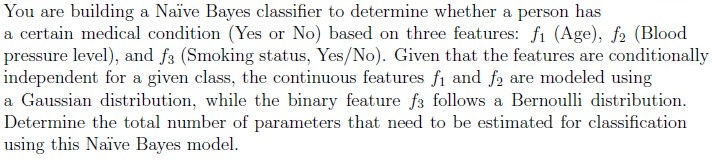
Parameter Count:
- Gaussian features: 2 parameters (μ, σ²) per feature per class.
- Bernoulli features: 1 parameter (p) per feature per class.
- Class priors: 1 parameter per class.
- Example: 2 Gaussian features + 1 Bernoulli feature + 2 classes → 11 parameters (not 12; class priors sum to 1).
Maximum Likelihood Estimation (MLE)
- Uniform Distribution: for .
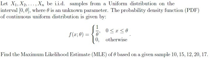
- MLE for θ: .
- Example: Sample → .
D. Ensemble Methods
Bagging (Bootstrap Aggregating)
Key Ideas:
- Trains multiple models on bootstrapped samples.
- Reduces variance (vs. individual learners).
- Parallelizable: Estimators are independent.
- Out-of-Bag (OOB) Error: ~33% of data is left out per tree (for large datasets).
Perceptron Algorithm
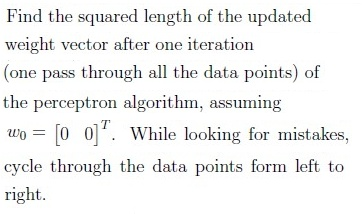
- Update Rule:
- Convergence: Guaranteed if data is linearly separable.
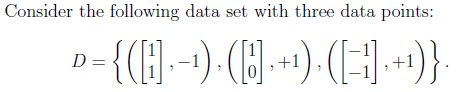
- Example: After 1 iteration, squared weight length = 1.
E. Neural Networks
Single-Layer Neural Network
Architecture:
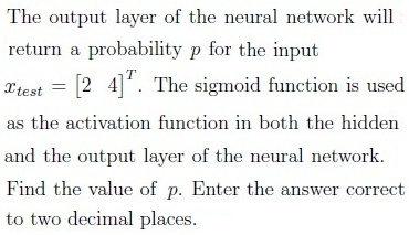
- Input layer → Hidden layer (2 neurons) → Output layer (sigmoid).
- Forward Pass:
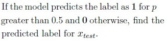
- Example: For , compute .
2. Key Equations
| Topic | Equation |
|---|---|
| Linear Regression | |
| Ridge Regression | |
| Lasso Regression | |
| SVM (Primal) | |
| SVM (Dual) | |
| AdaBoost Weight Update | |
| PCA | (where = eigenvectors of ) |
| Kernel PCA | (kernel matrix) |
| Perceptron Update | (if misclassified) |
| MLE (Uniform) | |
| Naïve Bayes (Gaussian) |
Graph 2: Unsupervised Learning & Probabilistic Models
Graph 3: Ensemble Methods & Neural Networks
4. Exam Tips
- k-NN: Higher
k→ smoother boundaries → lower LOOCV error. - Ridge/Lasso: Match vectors to (smaller → larger ).
- SVM: → hard margin; → soft margin.
- AdaBoost: Misclassified points get higher weights (e.g., 1/2 vs 1/6).
- PCA vs Kernel PCA: PCA is linear; Kernel PCA captures non-linear patterns.
- Naïve Bayes: Count parameters carefully (class priors sum to 1).
- Perceptron: Converges if data is linearly separable.
- Neural Networks: Compute hidden layer outputs step-by-step.