Home / Past papers / MLT Quiz 1 / this paper
IIT M FOUNDATION AN4 EXAM QPF4 16 JULY 2023 - 16 Jul 2023
Elapsed 00:00
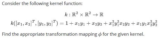





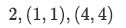
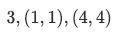


Select all true statements regarding standard PCA applied on a centered dataset.
- The variance of the dataset along the first principal component is maximum.
- The variance of the dataset along the first principal component is minimum.
- The first principal component is the unit norm eigenvector corresponding tothe largest eigenvalue of the covariance matrix.
- The first principal component is the unit norm eigenvector corresponding tothe smallest eigenvalue of the covariance matrix.

- The covariance matrix corresponding to this dataset has 30 non-zeroeigenvalues.
- The covariance matrix corresponding to this dataset has only four non-zeroeigenvalues.
- The residues will become zero after four rounds
- By utilizing four principal component vectors and their correspondingcoefficients, we have the ability to reconstruct the complete dataset using representatives.
Which of the following statements about kernel PCA is/are always true?





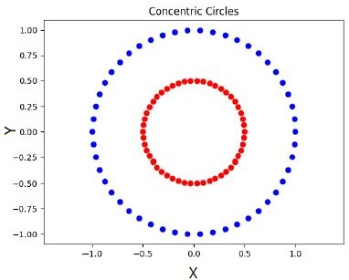
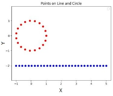
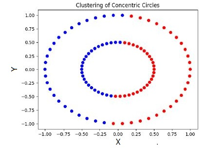
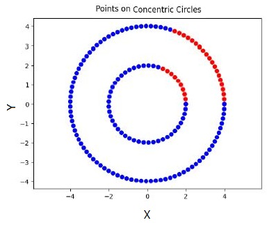
Which of the following statements is/are true?




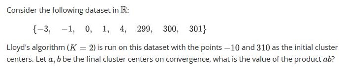


Concepts this paper tests
Auto-generated summary from the source site. Handy as a checklist; the lessons above explain each idea from scratch.
Summary of Core Topics, Concepts, Principles, and Equations
1. Kernel Functions and Transformation Mapping
- Kernel Functions: Functions that compute the dot product of the transformed input data in a higher-dimensional space.
- Transformation Mapping (): A function that maps input data into a higher-dimensional space.
- Example Kernel Function:
- Transformation Mapping for the Given Kernel:
2. K-means Clustering
- Algorithm: Iterative algorithm that partitions data into clusters.
Steps:
- Initialize centroids.
- Assign each data point to the nearest centroid.
- Recalculate centroids as the mean of the assigned points.
- Repeat until convergence.
Example:
- Points: , , ,
- Initial centroids: ,
- Final centroids after convergence: ,
3. Principal Component Analysis (PCA)
- Objective: Reduce the dimensionality of a dataset while preserving its variance.
Steps:
- Center the data.
- Compute the covariance matrix.
- Compute the eigenvectors and eigenvalues of the covariance matrix.
- Select the top eigenvectors (principal components).
Key Points:
- The first principal component has the maximum variance.
- The first principal component is the unit norm eigenvector corresponding to the largest eigenvalue of the covariance matrix.
Example:
- Dataset of 200 points in lying in a four-dimensional subspace.
- After PCA, the covariance matrix has only four non-zero eigenvalues.
4. Kernel PCA
- Objective: Extend PCA to non-linear datasets using kernel functions.
Key Points:
- The number of principal components can exceed the dimensionality of the original dataset.
- Valid kernel functions can be combined linearly with positive coefficients.
- Not all kernel functions are positive definite.
Example:
- Kernel function:
- Valid kernel function: where
5. Lloyd's Algorithm (K-means)
- Behavior: Minimizes within-cluster variance.
- Limitations: Cannot obtain clusters that do not minimize within-cluster variance, such as concentric circles or highly imbalanced clusters.
Example:
- Dataset:
- Initial centroids: ,
- Final centroids: ,
- Product of final centroids:
6. Bernoulli Distribution and Maximum Likelihood Estimation (MLE)
- Bernoulli Distribution: Models binary outcomes with parameter .
- MLE for : Estimates the parameter based on observed data.
Example:
- Dataset with 100 data points, MLE estimate for is 0.3.
- Number of zeros:
7. Beta Distribution and Bayesian Inference
- Beta Distribution: Prior and posterior distributions for the parameter of a Bernoulli distribution.
Example:
- Prior:
- Posterior:
- Number of zeros in the dataset: 40
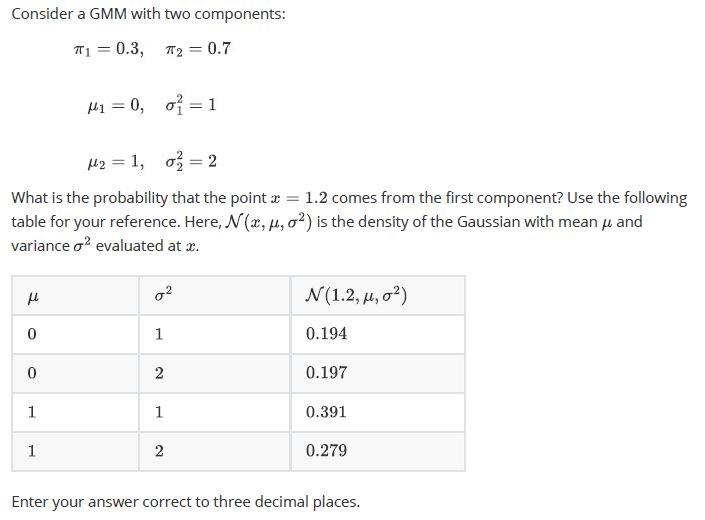
8. Gaussian Mixture Models (GMM)
- Objective: Model data as a mixture of Gaussian distributions.
- Probability Calculation: Use the Gaussian density function to compute the probability of a data point belonging to a component.
Example:
GMM with two components:
- , ,
- , ,
- Probability that comes from the first component: between 0.15 and 0.35