Home / Past papers / MLT End Term / this paper
IIT M IMPROVEMENT AN EXAM QIM3 13 Apr - 13 Apr 2025
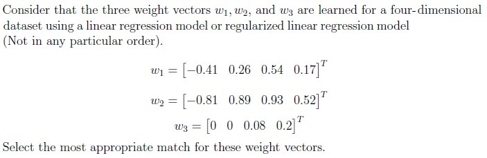
- It ensures that the dataset is normally distributed.
- It penalizes large coefficients to reduce overfitting.
- It forces more coefficients to be exactly zero, performing feature selection.
- It increases the variance of the model.
- The entropy of the node is maximum.
- The information gain at the node is negative.
- All samples at a node belong to the same class.
- The entropy of the node is 0.






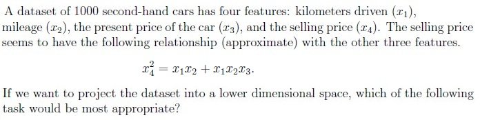
- Kernel PCA with a polynomial kernel of degree 2.
- Kernel PCA with a polynomial kernel of degree 3.
- Kernel PCA with a polynomial kernel of degree 4.
- Standard PCA
- TRUE
- FALSE
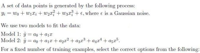
- Model 1 will have a higher bias than Model 2.
- Model 2 will have a lower variance than Model 1.
- Model 1 is more likely to underfit.
- Model 1 is more likely to overfit.






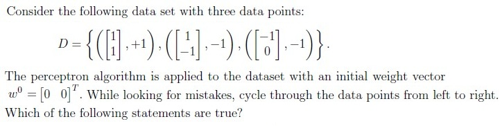






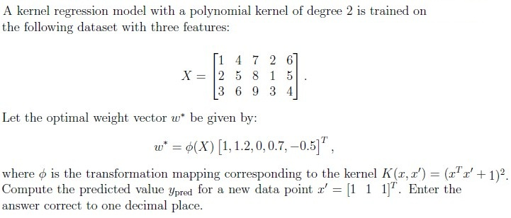
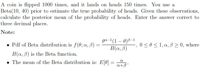
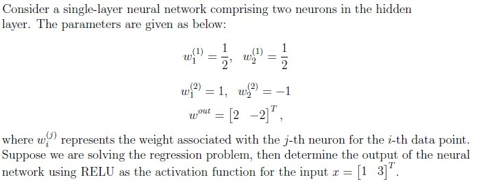
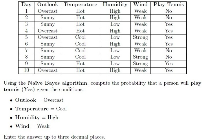 The following dataset represents different weather conditions and the corresponding decision on whether a person chooses to play tennis:

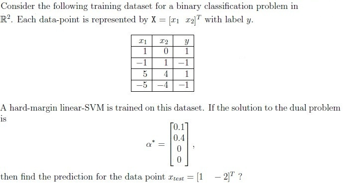
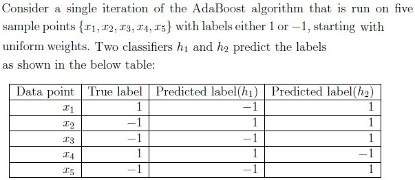


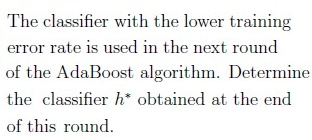




Answer key
- Q1 (MSQ, 2 marks): B
- Q2 (MSQ, 2 marks): C, D
- Q3 (MCQ, 3 marks): B
- Q4 (MCQ, 3 marks): A
- Q5 (MCQ, 2 marks): B
- Q6 (MCQ, 1 marks): A
- Q7 (MSQ, 3 marks): A, C
- Q8 (MSQ, 3 marks): B, D, E
- Q9 (MSQ, 4 marks): B, E
- Q10 (SA, 4 marks): 262.2 to 262.8
- Q11 (SA, 4 marks): 0.148 to 0.154
- Q12 (SA, 4 marks): 4
- Q13 (SA, 4 marks): 0.61 to 0.67
- Q14 (SA, 3 marks): 1
- Q15 (SA, 3 marks): 1
- Q16 (MCQ, 2 marks): A
- Q17 (MCQ, 3 marks): B
Concepts this paper tests
Auto-generated summary from the source site. Handy as a checklist; the lessons above explain each idea from scratch.
Here’s a structured summary of core topics, concepts, principles, and equations for the Diploma-Level Machine Learning Techniques exam, along with Mermaid knowledge graphs to visualize relationships.
1. Core Topics & Key Concepts
A. Supervised Learning
Linear Regression & Regularization
Ordinary Least Squares (OLS):
- Minimizes .
- Closed-form solution: .
Ridge Regression (L2 Regularization):
- Loss: .
- Penalizes large coefficients (reduces overfitting).
- Solution: .
Lasso Regression (L1 Regularization):
- Loss: .
- Forces sparse solutions (feature selection).
- Key Equation:
Logistic Regression
- Sigmoid function: .
- Decision boundary: if .
- Key Equation:
Support Vector Machines (SVM)
Hard-Margin SVM:
- Maximizes margin .
- Constraints: .
Soft-Margin SVM:
- Allows misclassification with slack variables .
- Primal problem:
Dual Problem:
- Solve for (Lagrange multipliers).
- Kernel trick: .
Key Properties:
- If : Correctly classified (non-support vector).
- If : Lies on margin (support vector).
- If : Misclassified or inside margin.
Decision Trees
Impurity Measures:
- Entropy: .
- Gini Index: .
Splitting Criteria:
- Information Gain (IG): .
Stopping Conditions:
- Node is pure (all samples same class, entropy = 0).
- Max depth reached.
Ensemble Methods
AdaBoost:
- Combines weak learners (slightly better than random guessing).
- Updates weights: Increase for misclassified samples.
- Final predictor: .
- Key Equation:
Perceptron Algorithm
- Updates weights when misclassified: .
- Converges if data is linearly separable.
B. Unsupervised Learning
Clustering (Lloyd’s Algorithm / K-Means)
Steps:
- Initialize centroids randomly.
- Assign points to nearest centroid.
- Recompute centroids as mean of assigned points.
- Key Equation:
Kernel PCA
- Projects data into higher-dimensional space using kernel .
- Polynomial Kernel: .
- Key Idea: Use kernel trick to avoid explicit transformation.
C. Probabilistic Models
Naïve Bayes
- Assumes feature independence given class: .
- Prediction: .
Bayesian Inference
- Prior: .
- Posterior: .
- Posterior Mean: .
D. Neural Networks
Single-Layer Neural Network
Activation Functions:
- ReLU: .
Forward Pass:
- Hidden layer: .
- Output: .
E. Dimensionality Reduction
PCA vs. Kernel PCA
- PCA: Linear projection to maximize variance.
- Kernel PCA: Nonlinear projection using kernel functions.
2. Key Equations Summary
| Topic | Equation |
|---|---|
| Ridge Regression | |
| Lasso Regression | |
| Logistic Regression | |
| SVM (Primal) | |
| SVM (Dual) | |
| Entropy | |
| Information Gain | |
| AdaBoost Weight | |
| K-Means Centroid | |
| Polynomial Kernel | |
| Beta Posterior Mean |
Graph 2: Unsupervised Learning
Graph 3: Probabilistic Models
Graph 4: Neural Networks
Graph 5: SVM Key Concepts
4. Exam-Specific Insights
Regularization (Q2, Q4):
- Ridge shrinks coefficients; Lasso performs feature selection.
Weight vectors:
- (sparse) → Lasso.
- (large coefficients) → Linear Regression.
- (moderate coefficients) → Ridge.
Decision Trees (Q3):
- Pure node: All samples same class or entropy = 0.
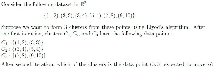
Clustering (Q5):
- Recompute centroids after assignment to find new clusters.
Kernel PCA (Q6):
- Relationship suggests degree 3 polynomial kernel.
AdaBoost (Q7, Q17, Q18):
- Weak learners must perform better than random (error < 50%).
- Lower training error → Higher weight in ensemble.
Bias-Variance Tradeoff (Q8):
- Model 1 (linear): High bias, low variance.
- Model 2 (high-degree polynomial): Low bias, high variance.
SVM Dual Problem (Q9):
- : Correctly classified.
- : On margin.
- : Misclassified or inside margin.
Perceptron (Q10):
- Converges for linearly separable data.
- Final weight vector depends on update order.
Kernel Regression (Q11):
- Use kernel to transform features implicitly.
- Prediction: .
Bayesian Inference (Q12):
- Posterior mean: .
Neural Networks (Q13):
- ReLU: .
- Output: Linear combination of hidden layer activations.
Naïve Bayes (Q14):
- Compute .
Logistic Regression (Q15):
- Predict if .
SVM Prediction (Q16):
- Dual solution defines support vectors.
- Prediction: .