Home / Past papers / MLT Quiz 1 / this paper
IIT M IMPROVEMENT AN EXAM QID4 26 Oct - 26 Oct 2025
- It always converges.
- It may fail to converge for an initialization while it may converge for otherinitialization.
- It is sensitive to outliers.
- The solution produced is always the optimal.

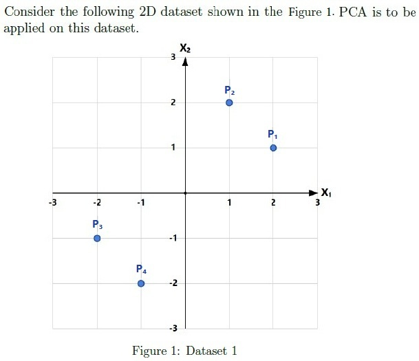
- There will be 50 non-zero eigenvalues of the covariance matrix.
- There will be 6 non-zero eigenvalues of the covariance matrix.
- Using the first 5 principal components, the dataset can be reconstructed withzero residue.
- The variance captured by the top 6 principal components equals the totalvariance of the dataset.
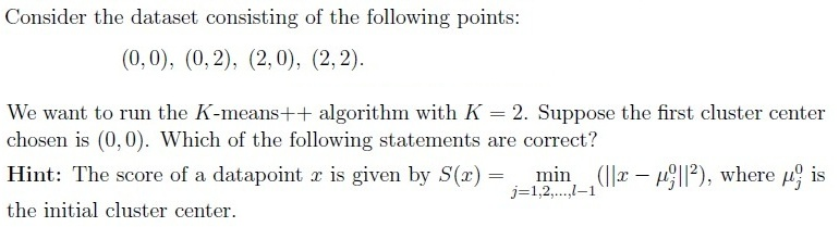
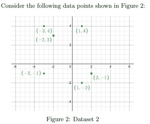
- The points (0, 2), (2, 0), and (2, 2) have the equal probability of being chosen asthe second cluster center.
- The probability of selecting (2, 2) as the second cluster center is twice that ofselecting (0, 2).
- If (2, 2) is chosen as the second cluster center, the algorithm will alwaysconverge in one iteration.
- The tie-breaking rule will affect the final cluster centers.
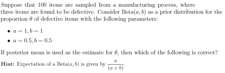
- Posterior mean for Beta(1, 1) is 0.039.
- Posterior mean for Beta(1, 1) is 0.03.
- Posterior mean for Beta(0.5, 0.5) is 0.025.
- Posterior mean for Beta(0.5, 0.5) is 0.034.















Answer key
- Q1 (MSQ, 2 marks): A, C
- Q2 (MSQ, 4 marks): B, D
- Q3 (MSQ, 4 marks): B, C, D
- Q4 (MSQ, 4 marks): A, D
- Q5 (MSQ, 3 marks): A, B, D
- Q6 (SA, 3 marks): 3
- Q7 (SA, 3 marks): 0.45 to 0.50
- Q8 (MCQ, 2 marks): B
- Q9 (SA, 2 marks): 4.5
- Q10 (SA, 2 marks): 0.5
- Q11 (MCQ, 3 marks): B
- Q12 (SA, 3 marks): 0.64 to 0.68
- Q13 (MCQ, 3 marks): A
- Q14 (SA, 2 marks): 1
Concepts this paper tests
Auto-generated summary from the source site. Handy as a checklist; the lessons above explain each idea from scratch.
Here's a comprehensive summary of the core topics, concepts, principles, and equations essential for the "Machine Learning Techniques" exam, derived from the provided questions.
Machine Learning Techniques Exam: Core Topics Summary
This exam focuses heavily on Unsupervised Learning techniques, particularly Clustering and Dimensionality Reduction, alongside foundational Mathematical Concepts from linear algebra, probability, and statistics.
1. Unsupervised Learning: Clustering
1.1 K-Means Clustering (Lloyd's Algorithm)
- Concept: An iterative partitioning algorithm that aims to partition data points into clusters, where each data point belongs to the cluster with the nearest mean (centroid).
Principles:
Algorithm Steps:
- Initialization: Choose initial cluster centroids.
- Assignment Step (E-step-like): Assign each data point to the cluster whose centroid is closest, typically using squared Euclidean distance.
- Update Step (M-step-like): Recalculate the centroids as the mean of all data points assigned to that cluster.
- Convergence: Repeat steps 2 and 3 until cluster assignments no longer change or centroids do not move significantly.
Properties:
- Convergence: Always converges in a finite number of iterations to a local optimum of the objective function.
- Sensitivity to Initialization: The final clustering result can vary significantly based on the initial placement of centroids.
- Sensitivity to Outliers: Highly sensitive to outliers due to its reliance on means and squared Euclidean distance, which heavily penalizes large distances.
- Optimality: Does not guarantee finding the global optimal clustering.
Equations:
Squared Euclidean Distance: For points and :
K-Means Objective Function (Sum of Squared Errors - SSE):
where is the set of points in cluster , and is the centroid of cluster .
Centroid Update:
1.2 K-Means++ Initialization
- Concept: A smart initialization technique for K-Means that selects initial centroids to be far apart, improving the chance of finding a better local optimum.
Principles:
- Randomly choose the first center from the data points.
- For each subsequent center, choose a data point with probability proportional to its squared distance from the closest existing center.
- This probabilistic selection biases towards choosing points that are far from already chosen centroids.
Equations:
Probability of selecting next center :
where and are the already chosen initial cluster centers.
1.3 Gaussian Mixture Models (GMM) and Expectation-Maximization (EM) Algorithm
- Concept: A probabilistic model that assumes data points are generated from a mixture of several Gaussian distributions with unknown parameters (means, covariances, and mixing weights). The EM algorithm is used to estimate these parameters.
Principles:
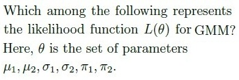
GMM Likelihood: For a dataset and Gaussian components, the likelihood function for parameters is:
where are the mixing coefficients (prior probabilities of components), and is the probability density function (PDF) of the -th Gaussian component.
EM Algorithm: An iterative optimization algorithm for finding maximum likelihood estimates of parameters in probabilistic models, especially when the model depends on unobserved latent variables.
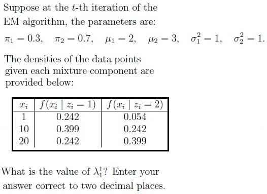
- E-step (Expectation): Calculate the "responsibilities" (posterior probabilities) that each data point belongs to each component, given the current parameter estimates.
- M-step (Maximization): Update the parameters (means, covariances, mixing weights) to maximize the expected log-likelihood found in the E-step.
Equations:
1D Gaussian PDF:
Responsibility (posterior probability for data point belonging to component ):
(This is the formula for as seen in textbooks).
2. Unsupervised Learning: Dimensionality Reduction
2.1 Principal Component Analysis (PCA)
- Concept: A linear dimensionality reduction technique that transforms data to a new coordinate system such that the greatest variance by any projection of the data lies on the first coordinate (first principal component), the second greatest variance on the second coordinate, and so on.
Principles:
- Covariance Matrix: PCA is based on the eigenvalue decomposition of the data's covariance matrix.
- Principal Components: The principal components are the eigenvectors of the covariance matrix, ordered by their corresponding eigenvalues in descending order.
- Variance Explained: Each eigenvalue represents the amount of variance captured along its corresponding principal component.
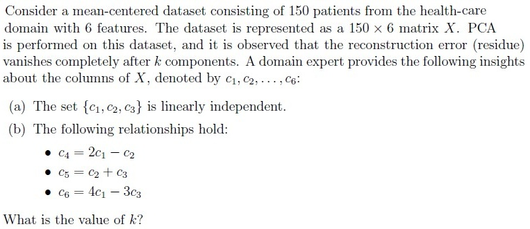
- Intrinsic Dimensionality: If a dataset inherently lies in a -dimensional linear subspace, then its covariance matrix will have non-zero eigenvalues, and principal components are sufficient to reconstruct the data with zero error.
- Reconstruction Error: When reducing dimensionality, the reconstruction error relates to the variance not captured by the selected principal components. Zero residue implies all variance is captured.
Equations:
Mean Vector: For a dataset where is the number of samples and is the number of features, the mean of feature is:
- Mean-Centered Data Matrix: (each row has mean subtracted).
Sample Covariance Matrix: For mean-centered data :
(Often is used in ML contexts for population covariance, or when treating as a population.) For a 2D dataset with points :
- Eigenvalue Decomposition: , where is an eigenvalue and is an eigenvector.
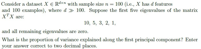
Proportion of Variance Explained (PVE) by -th principal component:
where is the eigenvalue for the -th principal component and is the total variance.
3. Kernel Functions
- Concept: Functions that compute the inner product between two vectors in a high-dimensional feature space, without explicitly transforming the data into that space (the "kernel trick"). Used in algorithms like SVMs and Kernel PCA to handle non-linear relationships.
Principles:
- A function is a valid kernel if it corresponds to an inner product in some high-dimensional feature space, i.e., for some mapping .
- Mercer's Theorem: Provides formal conditions for a function to be a valid kernel (the kernel matrix must be positive semi-definite).
Common Valid Kernels:
Radial Basis Function (RBF) / Gaussian Kernel:
where (or ) is a bandwidth parameter.
Polynomial Kernel:
where is a constant and is the degree of the polynomial.
Linear Kernel:
Non-Valid Kernels (Example):
- (absolute distance) is generally not a valid kernel as it does not typically correspond to an inner product.
4. Bayesian Inference (Beta-Binomial Model)
- Concept: A framework for updating beliefs about parameters of a distribution using observed data. The Beta-Binomial model is a common example of a conjugate prior relationship.
Principles:
Bayes' Theorem: Relates the posterior probability of a parameter () given data () to the likelihood of the data given the parameter and the prior probability of the parameter.
- Conjugate Prior: When the posterior distribution is in the same family as the prior distribution. For a Binomial likelihood, the Beta distribution is a conjugate prior.
- Beta Distribution: A continuous probability distribution defined on the interval , often used to model probabilities or proportions.
- Binomial Distribution: A discrete probability distribution of the number of successes in a sequence of independent yes/no experiments.
Equations:
- Beta Prior Distribution:
- Binomial Likelihood: Given successes in trials:
Beta Posterior Distribution: Given a prior and observing successes in trials, the posterior is:
Expected Value of a Beta Distribution: For :
Posterior Mean: The expected value of the posterior distribution, used as an estimate for :