Home / Past papers / MLT Quiz 1 / this paper

IIT M IMPROVEMENT AN EXAM QIB4 26 Oct - 26 Oct 2025

MLT Quiz 114 questions40 marks6 SA · 5 MSQ · 3 MCQImprovement / afternoon / QIB4

Elapsed 00:00

Q1MSQ2 marksselect all that apply

Which among the following is true with respect to the Lloyds’ algorithm?

It always converges.
It may fail to converge for an initialization while it may converge for otherinitialization.
It is sensitive to outliers.
The solution produced is always the optimal.

Q2MSQ4 marksselect all that apply

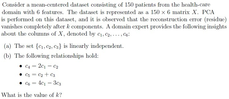
There will be 50 non-zero eigenvalues of the covariance matrix.
There will be 6 non-zero eigenvalues of the covariance matrix.
Using the first 5 principal components, the dataset can be reconstructed withzero residue.
The variance captured by the top 6 principal components equals the totalvariance of the dataset.

Q3MSQ4 marksselect all that apply

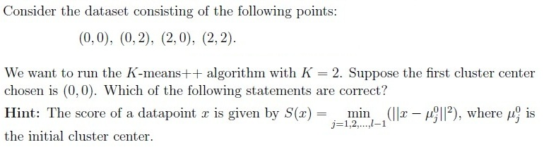
The points (0, 2), (2, 0), and (2, 2) have the equal probability of being chosen asthe second cluster center.
The probability of selecting (2, 2) as the second cluster center is twice that ofselecting (0, 2).
If (2, 2) is chosen as the second cluster center, the algorithm will alwaysconverge in one iteration.
The tie-breaking rule will affect the final cluster centers.

Q4MSQ4 marksselect all that apply

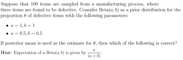
Posterior mean for Beta(1, 1) is 0.039.
Posterior mean for Beta(1, 1) is 0.03.
Posterior mean for Beta(0.5, 0.5) is 0.025.
Posterior mean for Beta(0.5, 0.5) is 0.034.

Q5MSQ3 marksselect all that apply

Which of the following are valid kernel functions? Select all that apply.

Q6SA3 marks

Your numeric answer:

Q7SA3 marks

Your numeric answer:

Comprehension passage - the questions below it refer to this

Based on the above data, answer the given subquestions. question figure

Q8MCQ2 marks

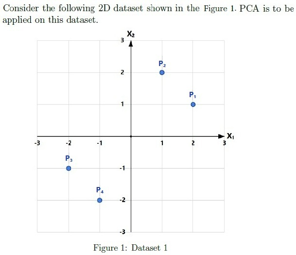
What is the covariance matrix of the dataset?

Q9SA2 marks

If standard PCA is performed on this dataset, what is the variance along the first principal component? Enter the answer correct to one decimal place.

Your numeric answer:

Q10SA2 marks

If standard PCA is performed on this dataset, what is the variance along the second principal component? Enter the answer correct to one decimal place.

Your numeric answer:

Comprehension passage - the questions below it refer to this

Based on the above data, answer the given subquestions. question figure

Q11MCQ3 marks

Q12SA3 marks

Your numeric answer:

Comprehension passage - the questions below it refer to this

Based on the above data, answer the given subquestions. question figure

Q13MCQ3 marks

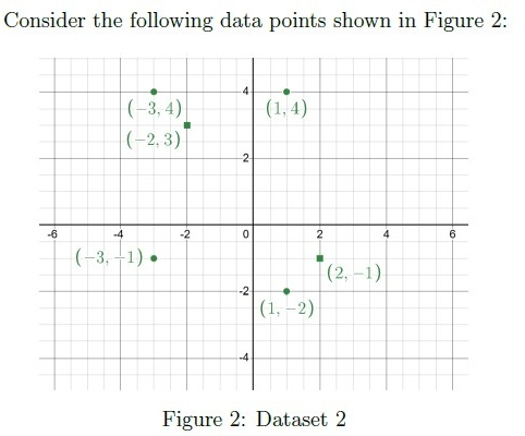
Perform K-means clustering with K = 2 and initial cluster centers at (−2, 3) and (2,−1). What are the final means of clusters after convergence?

Q14SA2 marks

Suppose we introduce a new data point (0, 0) to the existing dataset and perform K means with the same initial cluster centers. How many iterations would it require now for convergence?

Your numeric answer:

Answer key

Q1 (MSQ, 2 marks): A, C
Q2 (MSQ, 4 marks): B, D
Q3 (MSQ, 4 marks): B, C, D
Q4 (MSQ, 4 marks): A, D
Q5 (MSQ, 3 marks): A, B, D
Q6 (SA, 3 marks): 3
Q7 (SA, 3 marks): 0.45 to 0.50
Q8 (MCQ, 2 marks): B
Q9 (SA, 2 marks): 4.5
Q10 (SA, 2 marks): 0.5
Q11 (MCQ, 3 marks): B
Q12 (SA, 3 marks): 0.64 to 0.68
Q13 (MCQ, 3 marks): A
Q14 (SA, 2 marks): 1

Concepts this paper tests

Auto-generated summary from the source site. Handy as a checklist; the lessons above explain each idea from scratch.

Here’s a structured summary of core topics, concepts, principles, and equations for the Diploma-Level Machine Learning Techniques exam, along with Mermaid knowledge graphs to visualize relationships.

1. Core Topics & Key Concepts

A. Clustering (K-Means, K-Means++, Lloyd’s Algorithm)

Key Concepts:

Lloyd’s Algorithm (Standard K-Means):
- Iterative algorithm to minimize within-cluster sum of squares (WCSS).
- Convergence: Always converges (monotonically decreases WCSS), but may reach local optima.
- Sensitivity to Outliers: Yes (since it uses Euclidean distance).
- Optimality: Does not guarantee global optimum (depends on initialization).

K-Means++ Initialization:
- Goal: Spread initial centroids to improve convergence.
- Selection Probability: Proportional to squared distance from existing centroids:

P(x) = \frac{S(x)^2}{\sum_{i=1}^n S(x_i)^2}, \quad S(x) = \min_{j} \|x - \mu_j\|^2

Advantage: Reduces likelihood of poor clustering.

Convergence Criteria:
- Stops when centroids stabilize or max iterations reached.

Equations:

WCSS (Within-Cluster Sum of Squares):

\text{WCSS} = \sum_{i=1}^n \min_{\mu_j \in C} \|x_i - \mu_j\|^2

Centroid Update:

\mu_j = \frac{1}{|C_j|} \sum_{x_i \in C_j} x_i

B. Principal Component Analysis (PCA)

Key Concepts:

Dimensionality Reduction:
- Projects data onto orthogonal axes (principal components) that maximize variance.
- Intrinsic Dimensionality: If data lies in a $k$ -dimensional subspace of $\mathbb{R}^d$ , the first $k$ PCs capture all variance.

Eigenvalue Decomposition:
- Covariance matrix $\Sigma = X^T X$ (if data is centered).
- Eigenvalues ( $\lambda_i$ ): Represent variance along principal components.
- Eigenvectors: Principal components (directions of max variance).

Reconstruction Error:
- Zero if $k = \text{rank}(X)$ . Otherwise, residual error exists.

Proportion of Variance Explained:

\text{Variance}_i = \frac{\lambda_i}{\sum_{j=1}^d \lambda_j}

Equations:

Covariance Matrix:

\Sigma = \frac{1}{n} X^T X \quad (\text{if } X \text{ is centered})

PCA Projection:

Z = X W \quad \text{where } W = [w_1, w_2, ..., w_k]

( $w_i$ = eigenvectors of $\Sigma$ ).

Reconstruction:

\hat{X} = Z W^T

C. Bayesian Statistics (Beta-Binomial Model)

Key Concepts:

Beta Distribution (Prior for Proportions):
- Conjugate prior for Binomial likelihood.
- PDF:

\theta \sim \text{Beta}(a, b), \quad f(\theta) = \frac{\theta^{a-1} (1-\theta)^{b-1}}{B(a,b)}

Mean:

E[\theta] = \frac{a}{a + b}

Posterior Update:
- Given data $D = (k \text{ successes}, n-k \text{ failures})$ :

\theta | D \sim \text{Beta}(a + k, b + n - k)

Posterior Mean:

E[\theta | D] = \frac{a + k}{a + b + n}

Equations:

Posterior Parameters:

a_{\text{post}} = a + \text{successes}, \quad b_{\text{post}} = b + \text{failures}

D. Kernel Methods

Key Concepts:

Kernel Trick:
- Maps data to higher-dimensional space where linear separation is possible.
- Kernel Function: $K(x, y) = \phi(x)^T \phi(y)$ .

Valid Kernels (Mercer’s Condition):
- Must be symmetric and positive semi-definite.
- Examples:
  - Gaussian (RBF) Kernel:

K(x, y) = \exp\left(-\frac{\|x - y\|^2}{2\sigma^2}\right)

Polynomial Kernel:

K(x, y) = (x^T y + c)^d

Laplacian Kernel:

K(x, y) = \exp\left(-\frac{\|x - y\|}{\sigma}\right)

Invalid Kernel: $K(x, y) = |x - y|$ (not PSD).

E. Gaussian Mixture Models (GMM) & EM Algorithm

Key Concepts:

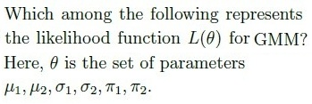
GMM Likelihood:
- Mixture of $K$ Gaussians:

p(x_i) = \sum_{k=1}^K \pi_k \mathcal{N}(x_i | \mu_k, \Sigma_k)

Log-Likelihood:

\log L(\theta) = \sum_{i=1}^n \log \left( \sum_{k=1}^K \pi_k \mathcal{N}(x_i | \mu_k, \Sigma_k) \right)

EM Algorithm:
- E-Step: Compute responsibilities ( $\gamma_{ik}$ ):

\gamma_{ik} = \frac{\pi_k \mathcal{N}(x_i | \mu_k, \Sigma_k)}{\sum_{j=1}^K \pi_j \mathcal{N}(x_i | \mu_j, \Sigma_j)}

M-Step: Update parameters:

\pi_k = \frac{1}{n} \sum_{i=1}^n \gamma_{ik}, \quad \mu_k = \frac{\sum_{i=1}^n \gamma_{ik} x_i}{\sum_{i=1}^n \gamma_{ik}}

\Sigma_k = \frac{\sum_{i=1}^n \gamma_{ik} (x_i - \mu_k)(x_i - \mu_k)^T}{\sum_{i=1}^n \gamma_{ik}}

Graph 2: PCA Concepts

Graph 3: Bayesian & GMM Concepts

Graph 4: Kernel Methods

3. Summary of Key Equations

Topic	Equation
K-Means WCSS	$\sum_{i=1}^n \min_{\mu_j} \\|x_i - \mu_j\\|^2$
PCA Variance	$\text{Variance}_i = \frac{\lambda_i}{\sum_j \lambda_j}$
Beta Posterior Mean	$\frac{a + k}{a + b + n}$
GMM Likelihood	$\prod_{i=1}^n \sum_{k=1}^K \pi_k \mathcal{N}(x_i \| \mu_k, \Sigma_k)$
EM Responsibility	$\gamma_{ik} = \frac{\pi_k \mathcal{N}(x_i \| \mu_k, \Sigma_k)}{\sum_j \pi_j \mathcal{N}(x_i \| \mu_j, \Sigma_j)}$
Gaussian Kernel	$\exp\left(-\frac{\\|x - y\\|^2}{2\sigma^2}\right)$

4. Exam Tips

PCA:
- If data lies in a $k$ -dimensional subspace, first $k$ PCs capture all variance.
- Reconstruction error is zero if $k = \text{rank}(X)$ .

K-Means++:
- Second centroid is chosen with probability proportional to $S(x)^2$ .

Bayesian:
- Posterior mean for $\text{Beta}(a, b)$ is $\frac{a}{a + b}$ after updating with data.

GMM:
- Likelihood involves a product of sums (not sum of products).

Kernels:
- $|x - y|$ is not a valid kernel. RBF, Polynomial, and Laplacian are valid.