Home / Past papers / MLT End Term / this paper
IIT M IMPROVEMENT FN EXAM QDD1 01 Sep - 01 Sep 2024

- 80%
- 60%
- 20%
- 15%


- Bagging → (2), (3); Boosting → (1), (4)
- Bagging → (1), (4); Boosting → (2), (3)
- Bagging → (1), (3); Boosting → (2), (4)
- Bagging → (2), (4); Boosting → (1), (3)
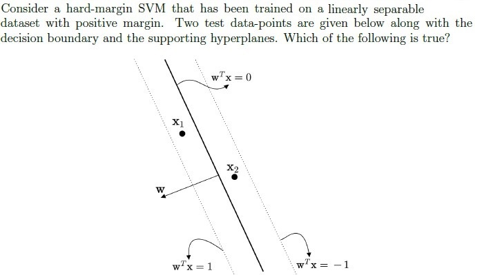
- The predicted labels for x1 and x2 are 1 and −1 respectively.
- The predicted labels for x1 and x2 are −1 and 1 respectively.
- The predicted label for both data-points is 1.
- The predicted label for both data-points is −1.





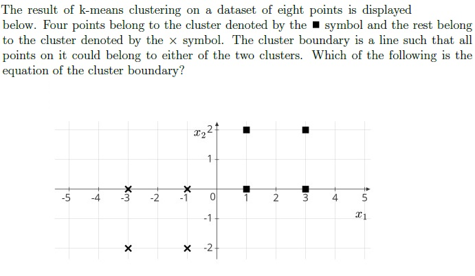
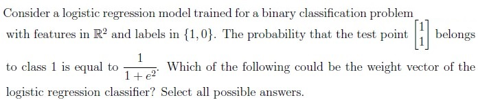
- 2x1 + x2 = 0
- x1 − 2x2 = 0
- x1 + x2 = 0
- x1 + 2x2 = 0




- 2
- 4
- 3
- 5
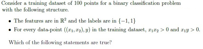
- The dataset is linearly separable with a positive margin.
- The perceptron algorithm will terminate after a finite number of iterationswhen trained on this dataset.
- The dataset is linearly separable, but the margin may be zero.
- The dataset is not linearly separable.



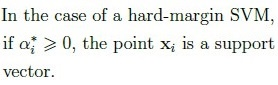
- TRUE
- FALSE
- TRUE
- FALSE
- TRUE
- FALSE






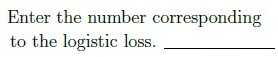



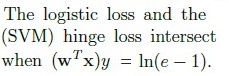

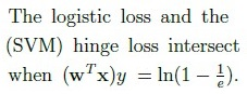
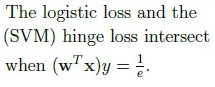
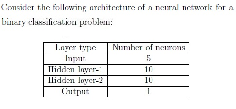
- Sigmoid
- Linear
- ReLU
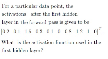
- ReLU
- Sigmoid



Answer key
- Q1 (MCQ, 3 marks): A
- Q2 (MCQ, 3 marks): A
- Q3 (MCQ, 3 marks): A
- Q4 (MCQ, 3 marks): A
- Q5 (MCQ, 3 marks): A
- Q6 (MCQ, 3 marks): A
- Q7 (SA, 3 marks): 0.4
- Q8 (SA, 3 marks): 30
- Q9 (SA, 3 marks): 0.26 to 0.37
- Q10 (MSQ, 3 marks): A, B
- Q11 (MSQ, 3 marks): A, B
- Q12 (MSQ, 3 marks): A, B
- Q13 (MCQ, 1 marks): A
- Q14 (MCQ, 1 marks): B
- Q15 (MCQ, 1 marks): B
- Q16 (SA, 0.5 marks): 2
- Q17 (SA, 0.5 marks): 1
- Q18 (SA, 0.5 marks): 0
- Q19 (SA, 0.5 marks): 3
- Q20 (SA, 0.5 marks): 0
- Q21 (SA, 0.5 marks): -1
- Q22 (SA, 0.5 marks): 3
- Q23 (SA, 0.5 marks): 2
- Q24 (SA, 0.5 marks): 4
- Q25 (SA, 0.5 marks): 1
- Q26 (MCQ, 1 marks): A
- Q27 (SA, 1 marks): 160
- Q28 (MCQ, 1 marks): A
- Q29 (MCQ, 1 marks): A
- Q30 (MCQ, 2 marks): A
Concepts this paper tests
Auto-generated summary from the source site. Handy as a checklist; the lessons above explain each idea from scratch.
Here’s a structured summary of core topics, concepts, principles, and equations essential for the exam, followed by Mermaid knowledge graphs to visualize relationships.
1. Core Topics & Concepts
A. Principal Component Analysis (PCA)
- Key Idea: Dimensionality reduction by projecting data onto orthogonal axes (principal components) that maximize variance.
Eigenvalues of Covariance Matrix:
- Represent variance along principal components.
- Total variance = Sum of all eigenvalues.
- Variance captured by top-k PCs = (Sum of top-k eigenvalues) / (Total variance).
- Equation:
(Where are eigenvalues, is dimensionality.)
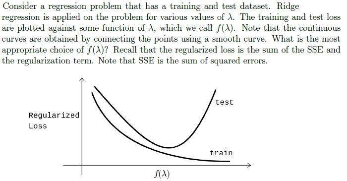
B. Regularization (Ridge Regression)
- Key Idea: Penalize large weights to prevent overfitting.
- Loss Function:
(SSE = Sum of Squared Errors, = regularization strength.)
Plot Interpretation:
- Training loss decreases with model complexity (lower ).
- Test loss has a U-shape; optimal minimizes it.
- Best : (balances scale for visualization).
C. Ensemble Methods (Bagging vs. Boosting)
| Feature | Bagging | Boosting |
|---|---|---|
| Base Models | Deep trees (high variance) | Decision stumps (high bias) |
| Execution | Parallel (independent models) | Sequential (corrects predecessors) |
| Combination | Averaging/voting | Weighted voting |
| Example Algorithms | Random Forest | AdaBoost, Gradient Boosting |
D. Support Vector Machines (SVM)
Hard-Margin SVM:
- Decision Boundary: .
- Supporting Hyperplanes: .
- Margin: .
- Distance between hyperplanes: .
Soft-Margin SVM:
- Slack Variables (): Allow misclassification.
- Objective:
(Subject to .)
Lagrange Multipliers ():
- .
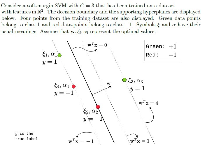
- Support Vectors: Points with .
KKT Conditions:
- If : Point is correctly classified outside margin.
- If : Point lies on margin ().
- If : Point is misclassified ().
E. Naive Bayes
- Class Conditional Independence:
(Features are independent given class .)
- Posterior Probability:
F. Clustering (k-Means)
Cluster Boundary: Perpendicular bisector between centroids.
- For centroids , boundary is:
Simplifies to a linear equation (e.g., ).
G. Logistic Regression
- Sigmoid Function:
- Probability of Class 1:
Weight Interpretation:
- If , then:
- Given , solve for .
H. Decision Trees & Information Gain
- Entropy:
(Where = proportion of class in set .)
- Information Gain:
(Where are child nodes.)
I. Kernels (Polynomial Kernel)
- Polynomial Kernel:
- Non-negativity: For even , kernel is always non-negative.
- Valid : 2, 4 (not odd degrees like 3, 5).
J. Neural Networks
Learnable Parameters:
- For layer with neurons and layer with neurons:
- Total Parameters (ignoring biases):
Activation Functions:
- Output Layer (Binary Classification): Sigmoid (for cross-entropy loss).
- Hidden Layers: ReLU (sparse activations), Sigmoid (vanishing gradients).
- ReLU Activation:
- If any activation in a layer is 0, the input to that neuron was ≤ 0.
K. Loss Functions
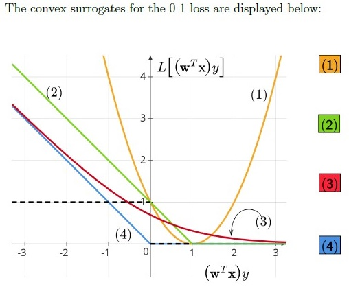
| Loss Function | Formula | Curve Color (from Q23-26) |
|---|---|---|
| Logistic Loss | Red (3) | |
| Hinge Loss (SVM) | Green (2) | |
| Perceptron Loss | Blue (4) | |
| Squared Loss | Yellow (1) |
L. Maximum Likelihood Estimation (MLE)
- Bernoulli MLE:
- Given and 10 successes (ones), total trials = 40.
- Zeros = Total trials - successes = 30.
M. Linear Regression (Gradient of SSE)
- SSE for One Data Point:
- Gradient w.r.t. :
Graph 2: Ensemble Methods
Graph 3: Neural Networks
Graph 4: Loss Functions
Graph 5: SVM Components
3. Key Equations Summary
| Topic | Equation |
|---|---|
| PCA Variance | |
| Ridge Regression | |
| SVM Margin | |
| SVM Objective | |
| Logistic Regression | |
| Entropy | |
| Information Gain | |
| Naive Bayes | |
| MLE (Bernoulli) | |
| Neural Net Parameters | |
| ReLU | |
| SSE Gradient |