Home / Past papers / MLP End Term / this paper
IIT M DEGREE AN EXAM QDB3 31 Aug 2025 - 31 Aug 2025
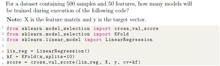
- 10
- 50
- 100
- 500
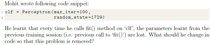
- Set ‘warm start=True’
- Combine training data from different training sessions
- Set ‘retain parameters=True’
- This problem can not be solved.

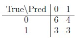
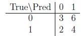
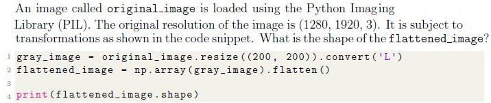
- (200, 200, 3)
- (40000, )
- (200, 200, 1)
- (40000, 3)





- The test is used to detect seasonality in a time series
- A low p-value (e.g., < 0.05) indicates the time series is non-stationary
- The test’s null hypothesis is that the time series is stationary
- A low p-value (e.g., < 0.05) indicates the time series is stationary





- liblinear
- lbfgs
- saga
- newton-cg






- The series is a product of a trend component and an error component only
- The series is a sum of a trend component, a seasonal component, and acyclical component
- The series is a product of a trend component, a seasonal component, and anerror component
- The series is a sum of a trend component, a seasonal component, and a errorcomponent

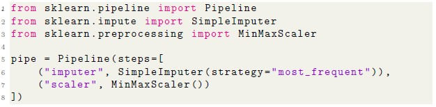

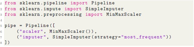

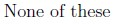

- Saves computation time by reusing results of expensive transformations wheninputs and parameters have not changed.
- Helps speed up repeated runs of cross-validation involving the sametransformation steps.
- Reduces CPU usage by running transformations in parallel threadsautomatically.
- Improves efficiency in hyperparameter search by avoiding redundantcomputations in pipeline steps.
- Guarantees better generalization performance on the test set.




- accuracy
- precision
- recall
- F-1 score

- The elbow method involves plotting the number of clusters against the inertiaand identifying a point where the decrease in inertia slows down.
- The elbow point represents the cluster count beyond which additional clustersdo not significantly improve the model fit.
- The metric used in the elbow method is the silhouette score.
- The elbow point is always the smallest number of clusters in the plot.
- The elbow method may sometimes be inconclusive if no clear bend is visible inthe curve.
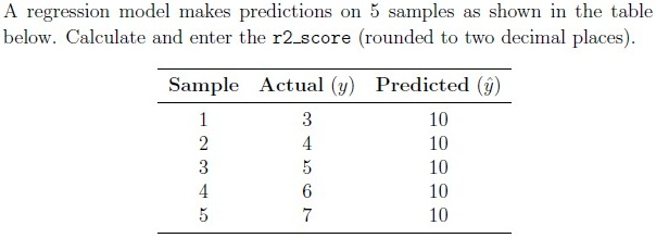
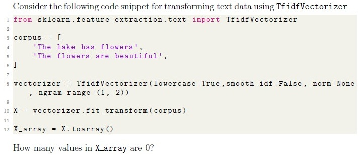
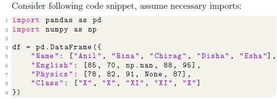
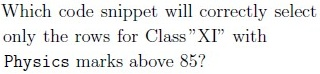
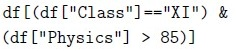
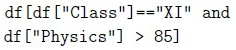
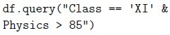
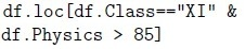
















Answer key
- Q1 (MCQ, 2 marks): A
- Q2 (MCQ, 2 marks): A
- Q3 (MCQ, 2 marks): A
- Q4 (MCQ, 2 marks): B
- Q5 (MCQ, 2 marks): A
- Q6 (MCQ, 2 marks): D
- Q7 (MCQ, 1 marks): A
- Q8 (MCQ, 1 marks): C
- Q9 (MCQ, 1 marks): A
- Q10 (MCQ, 3 marks): C
- Q11 (MSQ, 3 marks): A, B
- Q12 (MSQ, 2 marks): A, B, D
- Q13 (MSQ, 2 marks): A, B, C
- Q14 (MSQ, 2 marks): B, C, D
- Q15 (MSQ, 2 marks): A, B, E
- Q16 (SA, 3 marks): -12.5
- Q17 (SA, 3 marks): 10
- Q18 (MSQ, 1 marks): A, C
- Q19 (MCQ, 2 marks): A
- Q20 (MSQ, 2 marks): A, C
- Q21 (MCQ, 2 marks): D
- Q22 (MSQ, 2 marks): B, D
- Q23 (SA, 1 marks): 72
- Q24 (SA, 1 marks): 0.97 to 0.99
- Q25 (SA, 1 marks): 0.81 to 0.83
- Q26 (SA, 3 marks): 4.1 to 4.3
Concepts this paper tests
Auto-generated summary from the source site. Handy as a checklist; the lessons above explain each idea from scratch.
Here’s a structured summary of core topics, concepts, principles, and equations for the Diploma-Level Machine Learning Practice (Computer-Based Exam), along with Mermaid knowledge graphs to visualize relationships.
1. Core Topics & Concepts
A. Supervised Learning
1. Linear Regression & Cross-Validation
Key Concepts:
LinearRegressionfromsklearn.linear_model.K-Fold Cross-Validation (
KFoldfromsklearn.model_selection).- Splits data into
n_splitsfolds. - Trains model
n_splitstimes (each fold used once for validation).
- Splits data into
cross_val_scoreevaluates model performance across folds.
Equation:
- Linear Regression:
- Mean Squared Error (MSE):
Example:
from sklearn.linear_model import LinearRegression
from sklearn.model_selection import cross_val_score, KFold
lin_reg = LinearRegression()
kf = KFold(n_splits=10)
scores = cross_val_score(lin_reg, X, y, cv=kf)  # Trains 10 models
2. Perceptron & Warm Start
Key Concepts:
Perceptronfromsklearn.linear_model.Warm Start: Retains model weights between
fit()calls.- Useful for incremental learning.
Parameter:
Perceptron(max_iter=100, random_state=1729, warm_start=True)
3. Logistic Regression & Regularization
Key Concepts:
Elastic-Net Regularization: Combines L1 (Lasso) and L2 (Ridge) penalties.
- Controlled by
l1_ratio(0 = Ridge, 1 = Lasso).
- Controlled by
Solvers:
saga: Supports Elastic-Net.liblinear: Supports L1/L2 but not Elastic-Net.
Equation:
- Elastic-Net Penalty:
4. SGDRegressor & Loss Functions
Key Concepts:
Stochastic Gradient Descent (SGD):
- Optimizes loss functions incrementally.
Loss Functions:
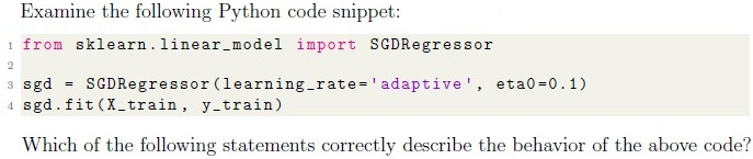
loss='huber': Less sensitive to outliers than squared loss.learning_rate='adaptive': Adjusts learning rate if loss doesn’t improve.
Parameters:
SGDRegressor(loss='huber', learning_rate='adaptive', eta0=0.1)
5. Evaluation Metrics
Key Concepts:
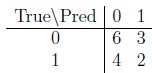
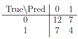
Confusion Matrix: TP, TN, FP, FN.
- Precision:
- Recall:
- F1-Score:
- R² Score:
- Imbalanced Data: Use Precision, Recall, F1 (not Accuracy).
B. Unsupervised Learning
1. K-Means Clustering
Key Concepts:
Elbow Method: Plots inertia (within-cluster sum of squares) vs. number of clusters.
- "Elbow" = optimal cluster count.
- Inertia:
Parameters:
KMeans(n_clusters=5, init='random', n_init=20, random_state=0)n_init: Number of initializations (avoids poor local minima).
2. Dimensionality Reduction (TF-IDF)
Key Concepts:
TF-IDF (Term Frequency-Inverse Document Frequency):
- Weights words by importance in a document vs. corpus.
Parameters:
TfidfVectorizer(lowercase=True, smooth_idf=False, norm=None, ngram_range=(1, 2))ngram_range=(1, 2): Includes unigrams and bigrams.
C. Time Series Analysis
1. Stationarity & ADF Test
Key Concepts:
Augmented Dickey-Fuller (ADF) Test:
- Null Hypothesis (): Time series is non-stationary.
- p-value < 0.05: Reject (series is stationary).
Decomposition:
- Multiplicative Model:
2. Collaborative Filtering
Key Concepts:
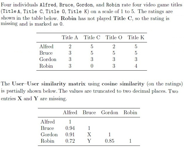
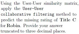
- User-User Similarity: Cosine similarity between user ratings.
- Prediction: Weighted average of similar users' ratings.
D. Data Preprocessing
1. Pipelines & Caching
Key Concepts:
Pipeline: Sequential data transformations.
from sklearn.pipeline import Pipeline
pipeline = Pipeline([
    ('imputer', SimpleImputer(strategy='most_frequent')),
    ('scaler', MinMaxScaler())
])
Caching (
memoryparameter):- Stores intermediate results to avoid recomputation.
- Useful for
GridSearchCVand cross-validation.
2. Handling Missing Data
Key Methods:
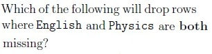
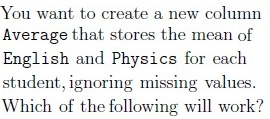
dropna(): Remove rows/columns with missing values.df.dropna(subset=["English", "Physics"], how="all") # Drops if both are NAfillna(): Impute missing values.mean(axis=1, skipna=True): Compute row-wise mean ignoringNaN.
E. Model Selection & Hyperparameter Tuning
1. GridSearchCV
Key Concepts:
- Exhaustive search over hyperparameter grid.
Parameters:
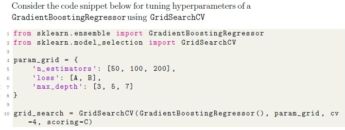
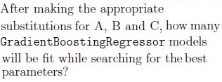
param_grid = { 'n_estimators': [50, 100, 200], 'loss': ['ls', 'lad', 'huber', 'quantile'], 'max_depth': [3, 5, 7] } grid_search = GridSearchCV(estimator, param_grid, cv=4, scoring='r2')- Total Models: Product of hyperparameter options (e.g., ).
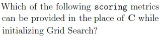
2. Scoring Metrics
Regression:
r2,neg_mean_absolute_error.
Classification:
precision,recall,f1,roc_auc.
F. Neural Networks (MLP)
1. MLPClassifier
Key Concepts:
- Hidden Layers: Specified as a tuple (e.g.,
(128, 64)= 2 layers). - Activation Functions:
relu,tanh,softmax. - Solvers:
adam,sgd,lbfgs.
- Hidden Layers: Specified as a tuple (e.g.,
Parameters:
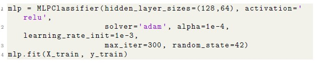
MLPClassifier(
    hidden_layer_sizes=(128, 64),
    activation='relu',
    solver='adam',
    alpha=1e-4,
    learning_rate_init=0.001,
    max_iter=300,
    random_state=42
)
Graph 2: Unsupervised Learning
Graph 3: Time Series Analysis
Graph 4: Model Tuning & Pipelines
Graph 5: Collaborative Filtering
3. Key Equations Summary
| Concept | Equation |
|---|---|
| Linear Regression | |
| MSE | |
| R² Score | |
| Elastic-Net Penalty | |
| Confusion Matrix Metrics | Precision = , Recall = |
| Cosine Similarity | |
| K-Means Inertia | |
| ADF Test Hypothesis | : Non-stationary, : Stationary |