Home / Past papers / MLP End Term / this paper
IIT M IMPROVEMENT AN EXAM QIC4 31 Aug - 31 Aug 2025
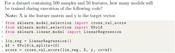
- 10
- 50
- 100
- 500
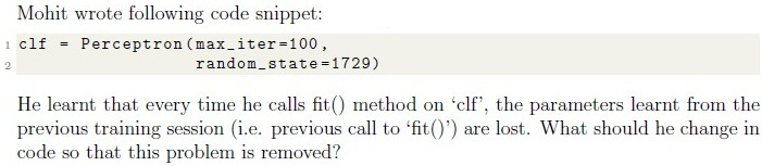
- Set ‘warm start=True’
- Combine training data from different training sessions
- Set ‘retain parameters=True’
- This problem can not be solved.

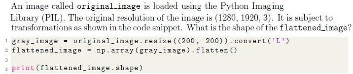
- (200, 200, 3)
- (40000, )
- (200, 200, 1)
- (40000, 3)





- The test is used to detect seasonality in a time series
- A low p-value (e.g., < 0.05) indicates the time series is non-stationary
- The test’s null hypothesis is that the time series is stationary
- A low p-value (e.g., < 0.05) indicates the time series is stationary





- liblinear
- lbfgs
- saga
- newton-cg






- The series is a product of a trend component and an error component only
- The series is a sum of a trend component, a seasonal component, and acyclical component
- The series is a product of a trend component, a seasonal component, and anerror component
- The series is a sum of a trend component, a seasonal component, and a errorcomponent

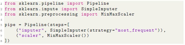

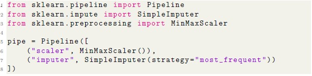


- Saves computation time by reusing results of expensive transformations wheninputs and parameters have not changed.
- Helps speed up repeated runs of cross-validation involving the sametransformation steps.
- Reduces CPU usage by running transformations in parallel threadsautomatically.
- Improves efficiency in hyperparameter search by avoiding redundantcomputations in pipeline steps.
- Guarantees better generalization performance on the test set.
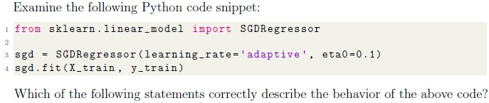




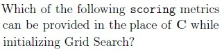
- accuracy
- precision
- recall
- F-1 score

- The elbow method involves plotting the number of clusters against the inertiaand identifying a point where the decrease in inertia slows down.
- The elbow point represents the cluster count beyond which additional clustersdo not significantly improve the model fit.
- The metric used in the elbow method is the silhouette score.
- The elbow point is always the smallest number of clusters in the plot.
- The elbow method may sometimes be inconclusive if no clear bend is visible inthe curve.
















Answer key
- Q1 (MCQ, 2 marks): A
- Q2 (MCQ, 2 marks): A
- Q3 (MCQ, 2 marks): A
- Q4 (MCQ, 2 marks): B
- Q5 (MCQ, 2 marks): A
- Q6 (MCQ, 2 marks): D
- Q7 (MCQ, 1 marks): A
- Q8 (MCQ, 1 marks): C
- Q9 (MCQ, 1 marks): A
- Q10 (MCQ, 3 marks): C
- Q11 (MSQ, 3 marks): A, B
- Q12 (MSQ, 2 marks): A, B, D
- Q13 (MSQ, 2 marks): A, B, C
- Q14 (MSQ, 2 marks): B, C, D
- Q15 (MSQ, 2 marks): A, B, E
- Q16 (SA, 3 marks): -12.5
- Q17 (SA, 3 marks): 10
- Q18 (MSQ, 1 marks): A, C
- Q19 (MCQ, 2 marks): A
- Q20 (MSQ, 2 marks): A, C
- Q21 (MCQ, 2 marks): D
- Q22 (MSQ, 2 marks): B, D
- Q23 (SA, 1 marks): 72
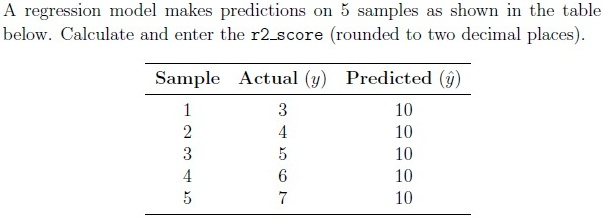
- Q24 (SA, 1 marks): 0.97 to 0.99
- Q25 (SA, 1 marks): 0.81 to 0.83
- Q26 (SA, 3 marks): 4.1 to 4.3
Concepts this paper tests
Auto-generated summary from the source site. Handy as a checklist; the lessons above explain each idea from scratch.
Here’s a structured summary of core topics, concepts, principles, and equations for the Diploma-Level Machine Learning Practice (Computer-Based Exam), along with Mermaid knowledge graphs to visualize relationships.
1. Core Topics & Concepts
A. Model Training & Evaluation
Key Concepts:
Cross-Validation (K-Fold)
- Splits data into
kfolds, trainsktimes (each fold as validation once). Equation:
- Inertia (for clustering):
- -score:
- Example: 10-fold CV trains 10 models (Q2).
- Splits data into
Model Persistence (
warm_start)- Retains weights between
.fit()calls (e.g.,Perceptron(warm_start=True)) (Q3).
- Retains weights between
Confusion Matrix
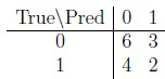
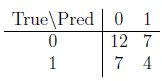
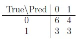
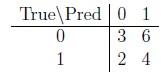
- Structure: | True\Pred | 0 | 1 | |-----------|---------|---------| | 0 | TN | FP | | 1 | FN | TP |
Metrics:
- Precision:
- Recall:
- F1:
- Use Case: Imbalanced data (e.g., rare disease detection) (Q15).
Evaluation Metrics for Imbalanced Data
- Avoid: Accuracy (misleading for rare classes).
- Use: Precision, Recall, F1, ROC-AUC (Q15).
B. Preprocessing & Feature Engineering
Image Processing
- Resize:
(1280, 1920, 3) → (200, 200)(grayscale). - Flatten:
(200, 200) → (40000,)(Q5). - Equation: Flattened shape = .
- Resize:
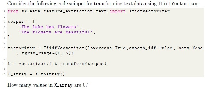
Text Vectorization (TF-IDF)
- TF-IDF:
- Sparsity: Most entries = 0 (Q18).
Handling Missing Data
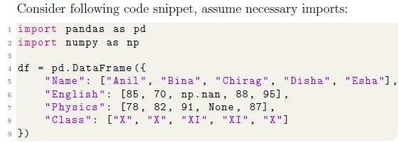
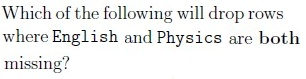
df.dropna(subset=["col1", "col2"], how="all")(drops rows where both are NaN) (Q20).- Imputation:
SimpleImputer(strategy="most_frequent")(Q12).
Feature Scaling
- MinMaxScaler: (scales to [0, 1]) (Q12).
C. Algorithms & Hyperparameters
Linear Models
SGDRegressor:
- Loss functions:
'huber','squared_error'(Q8, Q22). - Learning rate:
'adaptive'(reduces LR if loss plateaus) (Q14).
- Loss functions:
Logistic Regression:
- Elastic-net: regularization (Q9).
- Solver:
'saga'(supports elastic-net).
Neural Networks (MLP)
Hyperparameters:
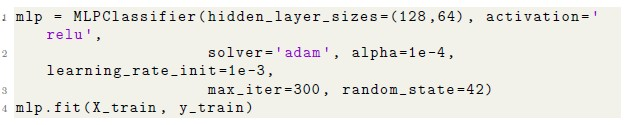
MLPClassifier( hidden_layer_sizes=(128, 64), # 2 hidden layers activation="relu", solver="adam", alpha=1e-4, # L2 regularization learning_rate_init=0.001, max_iter=300 )- Equation: Output = (Q6).
Clustering (K-Means)
- Elbow Method: Plot inertia vs. ; choose at the "elbow" (Q16).
- Inertia: Sum of squared distances to centroids.
Time Series
ADF Test:
- Null hypothesis: Time series is non-stationary (Q7).
- Interpretation: → stationary.
Decomposition:
- Multiplicative: (Q11).
Collaborative Filtering
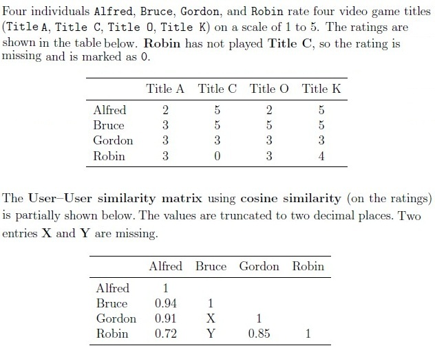
- Cosine Similarity:
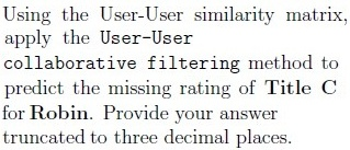
- Prediction: Weighted average of similar users' ratings (Q25–27).
D. Scikit-Learn Utilities
Pipelines
- Caching:
memory="path/to/cache"avoids recomputing transformations (Q13). Example:
Pipeline([
    ("imputer", SimpleImputer(strategy="most_frequent")),
    ("scaler", MinMaxScaler())
])
- Caching:
Grid Search
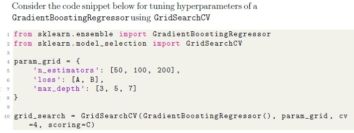
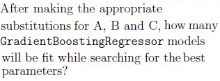
Total Models: Product of hyperparameter options (Q24).
- Example: 3 (
n_estimators) × 4 (loss) × 3 (max_depth) = 36 models.
- Example: 3 (
Scoring Metrics:
- Regression:
'neg_mean_squared_error','r2'. - Classification:
'f1','roc_auc'(Q23).
- Regression:
Graph 2: Preprocessing Workflow
Graph 3: Algorithm Selection
Graph 4: Time Series Analysis
Graph 5: Collaborative Filtering
3. Key Equations
| Concept | Equation |
|---|---|
| R² Score | |
| Inertia (K-Means) | |
| TF-IDF | |
| Cosine Similarity | |
| Elastic-Net Penalty | |
| ADF Test Null | : Time series is non-stationary |
4. Exam Tips
- Cross-Validation: Always count models as
n_splits(Q2). - Imbalanced Data: Avoid accuracy; use precision/recall/F1 (Q15).
- Hyperparameter Tuning: Total models = product of options (Q24).
- Text/Image Data: Flattening →
(height × width × channels,)(Q5). - Time Series: ADF → stationary (Q7).
- Collaborative Filtering: Cosine similarity for user-user predictions (Q25–27).