Home / Past papers / MLP End Term / this paper
Subject Name : 2023 Sep03: IIT M DIPLOMA ET1 EXAM - 03 Sep 2023
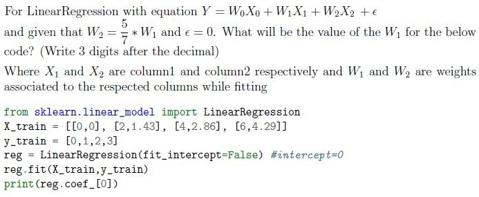
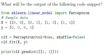
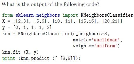
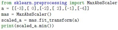 What will be the output of the following code:
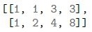
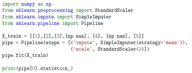 What will be the numerical value in the output array of the following code:
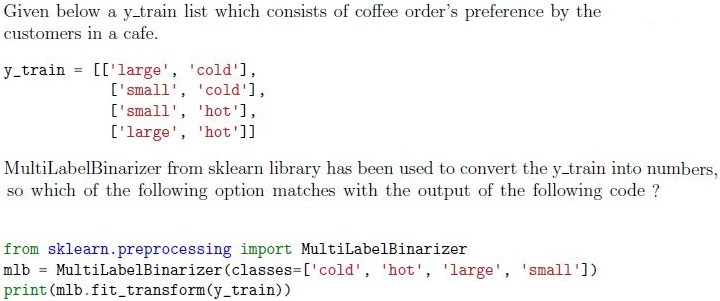




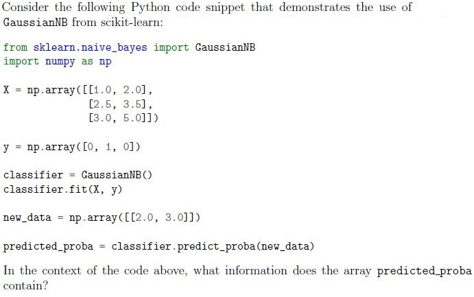
- The predicted classes for the new data points.
- The decision boundary values for the classes.
- The posterior probabilities of the classes for the new data points.
- The likelihood estimates for the new data points.
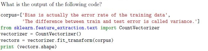
- (15,2)
- (2,3)
- (2,15)
- (15,3)
- Linear Regression
- Decision Tree
- K-means Clustering
- Support Vector Machine
- Complete Linkage
- Ward’s Linkage
- Single Linkage
- Average Linkage
- Distribution-based Clustering
- Density-based Clustering
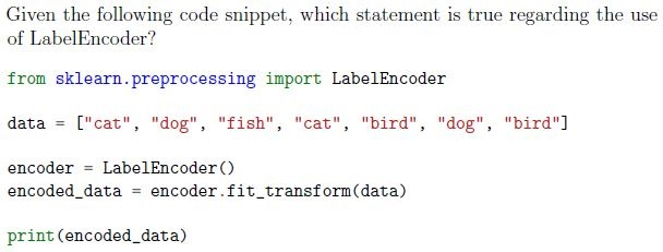





- MultinomialNB
- RandomForestRegressor
- LogisticRegressor
- SGDRegressor
- It is a technique used to minimize the adjusted loss function and avoidunderfitting.
- It helps in increasing the bias of the training model.
- It determines the rows to be selected as a training dataset.
- Elastic net regularization is a combination of L1 and L2 regularization both.
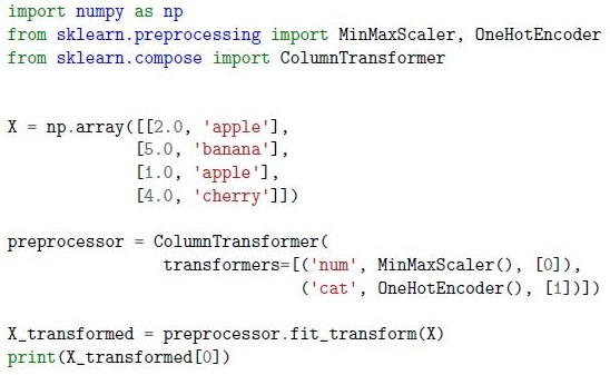 Given the following code snippet that preprocesses a dataset with both continuous and categorical features using sklearn.preprocessing tools, what will be the first row of the X transformed array after preprocessing?
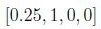


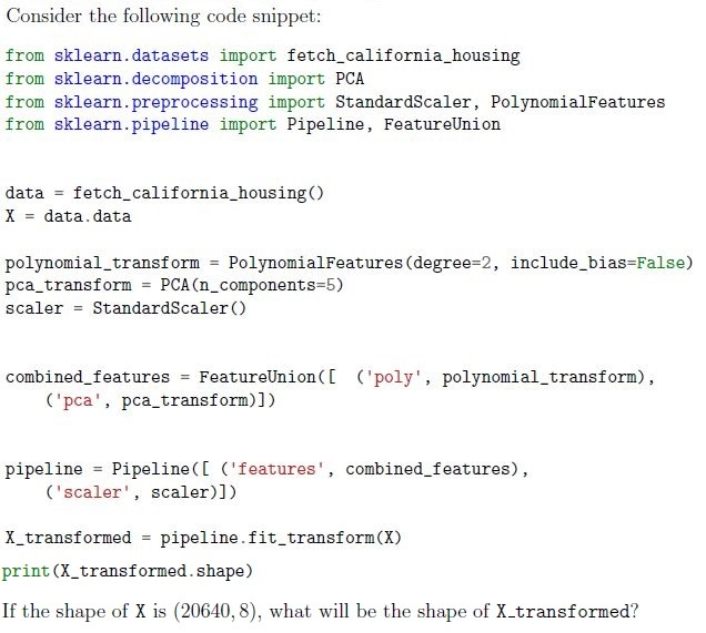
- (20640, 8)
- (20640, 5)
- (20640, 44)
- (20640, 49)
- Predict the mean or median of the target variable for all instances.
- Fit a complex mathematical function to the data.
- Randomly shuffle the target variable values to make predictions.
- Predict the sum of the input features for each instance.
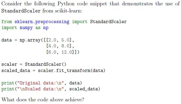
- It converts the numerical values in the data array to categorical labels.
- It standardizes the features in the data array to have zero mean and unitvariance.
- It applies a logarithmic transformation to the values in the data array.
- It removes the mean and scales the features in the data array to a specificrange.
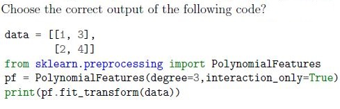
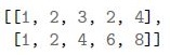


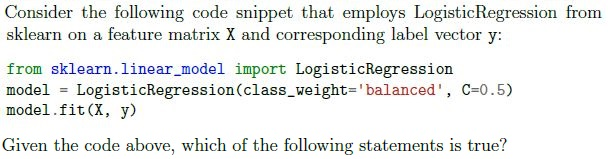





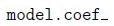



- Newton-CG
- SGD
- LBFGS
- Liblinear

- Increasing the number of neurons in hidden layers will always lead to bettermodel performance.
- Decreasing the number of neurons in hidden layers reduces the model’scapacity to capture complex patterns.
- The number of neurons in hidden layers does not significantly affect themodel’s performance.
- Finding the optimal number of neurons is a trial-and-error process and mayrequire experimentation.
- Number of hidden layers
- Number of neurons in input layer
- Learning rate
- Activation function
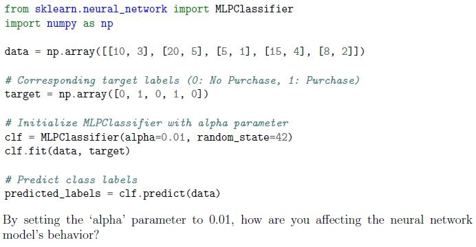 You’re working on a binary classification task using the ‘MLPClassifier’ to predict whether a customer will make a purchase based on their browsing behavior.You’re concerned about overfitting due to the complexity of the model. You decide to increase the ‘alpha’ parameter to control overfitting. The following code snippet shows the application of ‘MLPClassifier’:
- Increasing the model’s complexity to fit the training data more closely.
- Adding a stronger regularization term to the loss function, discouragingcomplex models.
- Making the model more sensitive to outliers and noise in the data.
- Adjusting the learning rate to control convergence speed.
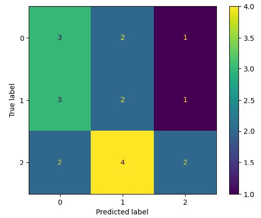 Using the confusion matrix given below. What is the precision score for the label (class) 1 ?
- KNeighborsClassifier with low values of n_neighbors produces complexdecision boundaries.
- KNeighborsClassifier with low values of n_neighbors produces smoothdecision boundaries.
- In KNeighborsClassifier the scale of the features(columns) can impact thedecision boundaries.
- None of these
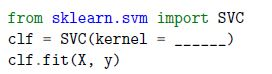 Fill in the missing parameter value in the following estimator that can be used to classify the data
- ‘lasso’
- ‘linear’,
- ‘rbf’,
- ‘scale’
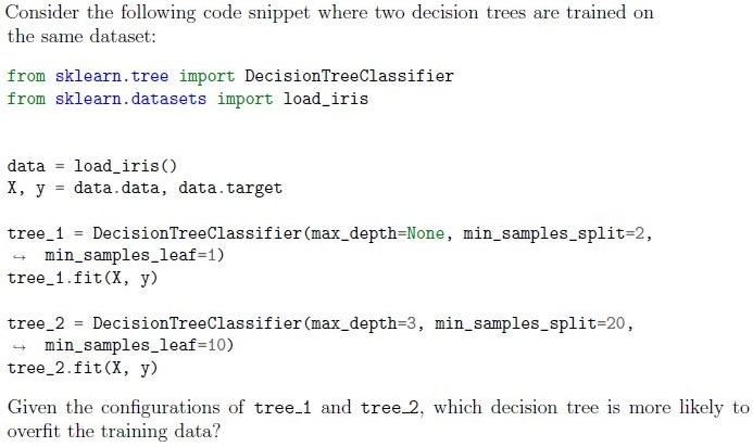


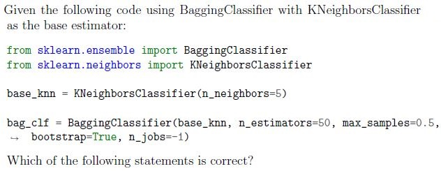














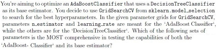

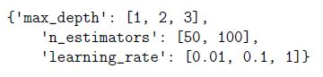

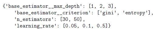
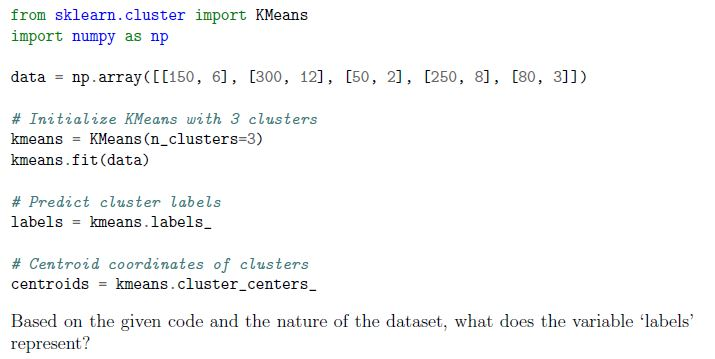 You’re working with a dataset of customer purchase behavior, including attributes “Total Amount Spent” and “Number of Items Purchased.” You decide to use K-means clustering to segment customers into groups based on these features. The following code snippet demonstrates the K-means clustering process:
- The total amount spent by each customer.
- The cluster assignments indicating which group each customer belongs to.
- The number of items purchased by each customer.
- The centroid coordinates of the clusters formed.
Answer key
- Q1 (SA, 2 marks): -1
- Q2 (SA, 2 marks): 3
- Q3 (MCQ, 2 marks): A
- Q4 (MCQ, 2 marks): C
- Q5 (MCQ, 2 marks): C
- Q6 (MCQ, 2 marks): C
- Q7 (MCQ, 2 marks): A
- Q8 (MCQ, 2 marks): A
- Q9 (MSQ, 3 marks): A, D
- Q10 (MSQ, 3 marks): A, D
- Q11 (MSQ, 3 marks): B, D
- Q12 (MCQ, 3 marks): A
- Q13 (MCQ, 3 marks): D
- Q14 (MCQ, 3 marks): A
- Q15 (MCQ, 3 marks): B
- Q16 (MCQ, 3 marks): B
- Q17 (MCQ, 3 marks): D
- Q18 (MCQ, 3 marks): A
- Q19 (MCQ, 3 marks): D
- Q20 (MCQ, 3 marks): D
- Q21 (MCQ, 3 marks): D
- Q22 (MCQ, 3 marks): B
- Q23 (SA, 3 marks): 0.327 to 0.333
- Q24 (SA, 3 marks): 0.25
- Q25 (SA, 3 marks): 1
- Q26 (SA, 3 marks): 1
- Q27 (MSQ, 4 marks): A, C
- Q28 (MSQ, 2 marks): B, C
- Q29 (MCQ, 4 marks): A
- Q30 (MCQ, 4 marks): C
- Q31 (MCQ, 4 marks): C
- Q32 (MCQ, 4 marks): A
- Q33 (MCQ, 4 marks): D
- Q34 (MCQ, 4 marks): B
Concepts this paper tests
Auto-generated summary from the source site. Handy as a checklist; the lessons above explain each idea from scratch.
Here’s a structured summary of core topics, concepts, principles, and equations essential for the Diploma Level: Machine Learning Practice (Computer-Based Exam). The exam covers data preprocessing, supervised/unsupervised learning, model evaluation, and neural networks, with a focus on scikit-learn implementations.
1. Core Topics & Concepts
A. Data Preprocessing
Key Concepts:
Scaling/Normalization
Standardization (
StandardScaler): Transforms data to have mean = 0 and variance = 1.- Formula:
Max-Abs Scaling (
MaxAbsScaler): Scales data to [-1, 1] by dividing by the maximum absolute value.- Formula:
Min-Max Scaling: Scales data to [0, 1].
- Formula:
Handling Missing Data
SimpleImputer: Replaces missing values with mean, median, or mode.- Example:
SimpleImputer(strategy='mean')
- Example:
Categorical Encoding
LabelEncoder: Converts categorical labels to numeric (0, 1, 2, ...).- Example:
encoder.fit_transform(["cat", "dog", "fish"])→[0, 1, 2]
- Example:
MultiLabelBinarizer: Converts categorical labels to binary vectors.Example:
mlb = MultiLabelBinarizer(classes=['cold', 'hot', 'large', 'small'])
mlb.fit_transform([['large', 'cold'], ['small', 'hot']])
Output:
[[1, 0, 1, 0], [0, 1, 0, 1]]
Polynomial Features
PolynomialFeatures: Generates interaction terms and polynomial features.- Example:
PolynomialFeatures(degree=2, interaction_only=True) - For input
[a, b], output includes[a, b, a*b](ifinteraction_only=True).
- Example:
Pipelines & Feature Unions
Pipeline: Chains multiple preprocessing steps.Example:
pipe = Pipeline([
    ('impute', SimpleImputer(strategy='mean')),
    ('scale', StandardScaler())
])
FeatureUnion: Combines multiple feature transformations.Example:
combined = FeatureUnion([
    ('poly', PolynomialFeatures(degree=2)),
    ('pca', PCA(n_components=2))
])
B. Supervised Learning
Key Algorithms & Concepts:
Linear Models
Linear Regression:
- Equation:
fit_intercept=False→ No bias term ().- Logistic Regression:
- Predicts probabilities (not classes directly).
predict_proba()→ Returns class probabilities.Regularization:
C(inverse of regularization strength): SmallerC→ stronger regularization.penalty='l1'(Lasso) or'l2'(Ridge).
Solvers:
liblinear: Good for small datasets + L1/L2.sag,saga: Good for large datasets.lbfgs,newton-cg: Default for multiclass.
Naive Bayes
GaussianNB: Assumes features follow a normal distribution.
predict_proba()→ Returns posterior probabilities.
k-Nearest Neighbors (KNN)
Hyperparameters:
n_neighbors: Low value → complex boundaries (prone to overfitting).weights='uniform'(all neighbors equal) or'distance'(weight by inverse distance).metric='euclidean'(default) or'manhattan'.
- Scaling matters: Features should be scaled (e.g.,
StandardScaler).
Support Vector Machines (SVM)
Kernel Trick: Transforms data into higher dimensions.
kernel='linear','rbf','poly'.
- Regularization:
Ccontrols margin strictness.
Neural Networks (MLP)
MLPClassifier:
hidden_layer_sizes=(n1, n2): Number of neurons in hidden layers.activation='relu','tanh','logistic'.alpha: L2 regularization (higher → more regularization).solver='adam'(default),'sgd','lbfgs'.
Overfitting Control:
- Increase
alpha→ stronger regularization. - Reduce hidden layer size → simpler model.
- Increase
C. Unsupervised Learning
Key Algorithms & Concepts:
Clustering
K-Means:
- Assigns points to K clusters by minimizing within-cluster variance.
n_clusters=K: Number of clusters.labels_: Cluster assignments for each point.cluster_centers_: Coordinates of centroids.
Hierarchical Clustering:
Linkage Methods:
complete(max distance),average,single(min distance),ward(min variance).
Dimensionality Reduction
PCA (Principal Component Analysis):
- Reduces features to n_components principal components.
PCA(n_components=2)
D. Model Evaluation
Key Metrics & Concepts:
Confusion Matrix
- Structure: | | | Predicted 0 | Predicted 1 | |---------------|------------------|------------------| | Actual 0 | True Negative (TN) | False Positive (FP) | | Actual 1 | False Negative (FN) | True Positive (TP) |
- Precision (for class 1):
- Recall (Sensitivity):
- F1-Score:
Regularization
- L1 (Lasso): Encourages sparsity (some weights = 0).
- L2 (Ridge): Penalizes large weights.
- Elastic Net: Combination of L1 + L2.
Bias-Variance Tradeoff
- High Bias (Underfitting): Model is too simple.
- High Variance (Overfitting): Model is too complex.
- Regularization helps reduce variance.
E. Ensemble Methods
Key Concepts:
Bagging (Bootstrap Aggregating)
BaggingClassifier: Trains multiple models on random subsets of data.Example:
BaggingClassifier(base_estimator=KNeighborsClassifier(), n_estimators=10)max_samples=0.5: Each estimator uses 50% of samples.
Random Forest
RandomForestClassifier:n_estimators: Number of trees.max_features: Features considered for splits (default=sqrt(n_features)).- Diversity: Achieved via random feature subsets and bootstrapping.
F. Text Feature Extraction
Key Concepts:
CountVectorizer
- Converts text to word-count matrix.
fit_transform(corpus)→ Returns(n_documents, n_unique_words)matrix.
TF-IDF (Term Frequency-Inverse Document Frequency)
- Weights words by importance (common words get lower weights).
2. Key Equations
| Concept | Equation |
|---|---|
| Standard Scaling | |
| Max-Abs Scaling | |
| Min-Max Scaling | |
| Linear Regression | |
| Logistic Regression (Sigmoid) | |
| Precision | |
| Recall | |
| F1-Score | |
| L1 Regularization (Lasso) | |
| L2 Regularization (Ridge) | |
| Polynomial Features (Degree 2) |
Graph 2: Supervised Learning Algorithms
Graph 3: Unsupervised Learning
Graph 4: Model Evaluation & Regularization
Graph 5: Ensemble Methods
4. Exam Tips
Focus Areas:
- Data Preprocessing: Scaling, encoding, imputation, pipelines.
- Supervised Learning: Logistic Regression, KNN, SVM, Neural Networks.
- Unsupervised Learning: K-Means, Hierarchical Clustering, PCA.
- Model Evaluation: Confusion matrix, precision/recall, regularization.
- Ensemble Methods: Bagging, Random Forest.
Common Pitfalls:
- Scaling: Always scale features for KNN, SVM, and neural networks.
- Regularization: Lower
Cin LogisticRegression/SVM = stronger regularization. - K-Means: Initialize with
n_clustersand checklabels_/cluster_centers_. - PolynomialFeatures:
interaction_only=Trueexcludes higher-degree terms for single features.
- Code Snippets to Remember: ```python # StandardScaler scaler = StandardScaler() scaled_data = scaler.fit_transform(data)
# K-Means kmeans = KMeans(n_clusters=3) kmeans.fit(data) labels = kmeans.labels_
# Logistic Regression with L1 model = LogisticRegression(penalty='l1', solver='liblinear')
# Pipeline pipe = Pipeline([ ('impute', SimpleImputer()), ('scale', StandardScaler()), ('model', LogisticRegression()) ]) ```
This summary covers 90% of the exam content. Focus on scikit-learn implementations, preprocessing steps, and model evaluation metrics for high scores!