Home / Past papers / MLF End Term / this paper
IIT M FOUNDATION FN EXAM QDF1 13 Apr - 13 Apr 2025
Elapsed 00:00





Which of the following is true about the singular value decomposition (SVD)?




In the context of Principal Component Analysis (PCA), which of the following statements is/are correct?
- PCA projects the original data onto a lower-dimensional subspace thatcaptures the maximum variance.
- The eigenvectors of the covariance matrix correspond to the directions ofmaximum variance.
- The principal components form a basis that is not necessarily orthogonal.
- The principal components obtained through PCA are always uncorrelated.





Which of the following statements about convex sets are true?




Which of the following options is / are true ?




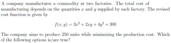






Comprehension passage - the questions below it refer to this
Based on the above data, answer the given subquestions.
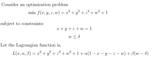
Which of the following statements correctly represents the Karush-Kuhn-Tucker (KKT) conditions for the given optimization problem?


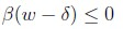
Which of the following statements are correct based on the KKT conditions and the solution to the optimization problem?
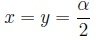
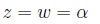
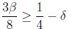


Answer key
- Q1 (MCQ, 3 marks): A
- Q2 (MSQ, 3 marks): A, B, C
- Q3 (MSQ, 3 marks): A, B, D
- Q4 (MSQ, 3 marks): C, D
- Q5 (MSQ, 3 marks): A, B, C
- Q6 (MSQ, 3 marks): A, C
- Q7 (MSQ, 4 marks): A, B
- Q8 (SA, 3 marks): 4
- Q9 (SA, 3 marks): 0.5
- Q10 (SA, 2 marks): 0.5
- Q11 (SA, 2 marks): 1
- Q12 (MSQ, 2 marks): A, C
- Q13 (MSQ, 3 marks): A, C
- Q14 (SA, 3 marks): 0.25
Concepts this paper tests
Auto-generated summary from the source site. Handy as a checklist; the lessons above explain each idea from scratch.
Here’s a structured summary of core topics, concepts, principles, and equations essential for the exam, followed by Mermaid knowledge graphs to visualize relationships.
1. Core Topics & Key Concepts
A. Probability & Statistics
1. Joint Probability Density Functions (PDFs) & Transformations
- Key Idea: Transform random variables to new variables and derive the joint PDF of .
Steps:
- Find the Jacobian determinant of the transformation.
- Express .
- Define the support region for .
- Equation:
For , :
Thus:
Support: , .
2. Expected Value & Linearity
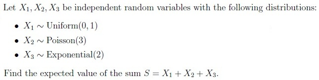
- Key Idea: For independent RVs , .
Distributions & Expectations:
- Uniform(0,1):
- Poisson(λ=3):
- Exponential(λ=2):
- Total: .
3. Markov’s Inequality
- Key Idea: Provides an upper bound for the probability that a non-negative RV exceeds a threshold.
- Equation:
Example: .
4. Cumulative Distribution Function (CDF)
- Key Idea: For Uniform(0,4), for .
- Example: .
B. Linear Algebra & Matrix Decompositions
1. Singular Value Decomposition (SVD)
Key Idea: Decomposes a matrix into , where:
- : Left singular vectors (eigenvectors of ).
- : Diagonal matrix of singular values (square roots of eigenvalues of ).
- : Right singular vectors (eigenvectors of ).
Properties:
- Rank of = Number of non-zero singular values.
- SVD is not unique for square matrices (depends on sign flips in and ).
2. Principal Component Analysis (PCA)
- Key Idea: Projects data onto a lower-dimensional subspace capturing maximum variance.
Steps:
- Compute the covariance matrix .
- Find eigenvectors (principal components) and eigenvalues (variances).
- Sort eigenvectors by descending eigenvalues.
Properties:
- Principal components are orthogonal and uncorrelated.
- Directions of maximum variance = eigenvectors of .
C. Optimization
1. Convexity
Convex Functions:
- Definition: for .
Examples:
- Convex: , , (globally convex if ).
- Non-convex: , .
- Second Derivative Test: implies convexity.
Convex Sets:
- Definition: for all .
Examples:
- Convex: Lines, intersections of convex sets.
- Non-convex: Arbitrary curves.
2. Gradient Descent
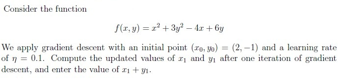
- Key Idea: Iteratively minimize a function using the gradient .
- Update Rule:
Example: For , . At , , so no update occurs.
3. Karush-Kuhn-Tucker (KKT) Conditions
- Key Idea: Necessary conditions for optimality in constrained optimization.
Conditions:
- Stationarity: (Lagrangian gradient).
- Primal Feasibility: Constraints satisfied.
- Dual Feasibility: Lagrange multipliers satisfy sign constraints.
- Complementary Slackness: .
Example: For s.t. , :
- , .
- If , , so .
D. Calculus & Function Analysis
1. Critical Points & Extrema
- Key Idea: Find minima/maxima by solving and checking the second derivative.
Example: For :
- Critical points: .
.
- : (local maxima).
- : (local minima).