Home / Past papers / MLF End Term / this paper

IIT M FOUNDATION FN EXAM QDF2 13 Apr - 13 Apr 2025

MLF End Term14 questions40 marks8 MSQ · 5 SA · 1 MCQFoundation / forenoon / QDF2

Elapsed 00:00

Q1MCQ3 marks

Q2MSQ3 marksselect all that apply

Which of the following is true about the singular value decomposition (SVD)?

Q3MSQ3 marksselect all that apply

In the context of Principal Component Analysis (PCA), which of the following statements is/are correct?

PCA projects the original data onto a lower-dimensional subspace thatcaptures the maximum variance.
The eigenvectors of the covariance matrix correspond to the directions ofmaximum variance.
The principal components form a basis that is not necessarily orthogonal.
The principal components obtained through PCA are always uncorrelated.

Q4MSQ3 marksselect all that apply

Q5MSQ3 marksselect all that apply

Which of the following statements about convex sets are true?

Q6MSQ3 marksselect all that apply

Which of the following options is / are true ?

Q7MSQ4 marksselect all that apply

Q8SA3 marks

Your numeric answer:

Q9SA3 marks

Your numeric answer:

Q10SA2 marks

Your numeric answer:

Q11SA2 marks

Your numeric answer:

Comprehension passage - the questions below it refer to this

Based on the above data, answer the given subquestions. question figure

Q12MSQ2 marksselect all that apply

Which of the following statements correctly represents the Karush-Kuhn-Tucker (KKT) conditions for the given optimization problem?

Q13MSQ3 marksselect all that apply

Which of the following statements are correct based on the KKT conditions and the solution to the optimization problem?

Q14SA3 marks

Your numeric answer:

Answer key

Q1 (MCQ, 3 marks): A
Q2 (MSQ, 3 marks): A, B, C
Q3 (MSQ, 3 marks): A, B, D
Q4 (MSQ, 3 marks): C, D
Q5 (MSQ, 3 marks): A, B, C
Q6 (MSQ, 3 marks): A, C
Q7 (MSQ, 4 marks): A, B
Q8 (SA, 3 marks): 4
Q9 (SA, 3 marks): 0.5
Q10 (SA, 2 marks): 0.5
Q11 (SA, 2 marks): 1
Q12 (MSQ, 2 marks): A, C
Q13 (MSQ, 3 marks): A, C
Q14 (SA, 3 marks): 0.25

Concepts this paper tests

Auto-generated summary from the source site. Handy as a checklist; the lessons above explain each idea from scratch.

Here’s a structured summary of core topics, concepts, principles, and equations essential for the exam, followed by Mermaid knowledge graphs to visualize relationships.

1. Core Topics & Key Concepts

A. Probability & Statistics

Joint Probability Density Function (PDF)
- Definition: $f_{X,Y}(x,y)$ for joint distribution of $X$ and $Y$ .
- Transformation of Variables:
  - Given $U = g_1(X,Y)$ , $V = g_2(X,Y)$ , find $f_{U,V}(u,v)$ using the Jacobian determinant:

f_{U,V}(u,v) = f_{X,Y}(x,y) \cdot |J|^{-1}, \quad \text{where } J = \begin{vmatrix} \frac{\partial x}{\partial u} & \frac{\partial x}{\partial v} \\ \frac{\partial y}{\partial u} & \frac{\partial y}{\partial v} \end{vmatrix}

Example: For $U = X + Y$ , $V = X - Y$ , solve for $X$ and $Y$ in terms of $U$ and $V$ , then compute $|J|$ .

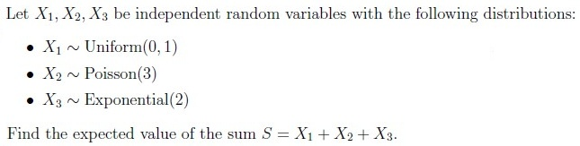
Expected Value & Linearity
- For independent RVs $X_1, X_2, X_3$ :

E[X_1 + X_2 + X_3] = E[X_1] + E[X_2] + E[X_3]

Distributions:
- Uniform( $a,b$ ): $E[X] = \frac{a+b}{2}$
- Poisson( $\lambda$ ): $E[X] = \lambda$
- Exponential( $\lambda$ ): $E[X] = \frac{1}{\lambda}$

Markov’s Inequality
- For non-negative RV $X$ and $a > 0$ :

P(X \geq a) \leq \frac{E[X]}{a}

Cumulative Distribution Function (CDF)
- For Uniform( $a,b$ ):

F_X(x) = \frac{x - a}{b - a}, \quad a \leq x \leq b

B. Linear Algebra & Matrix Decompositions

Singular Value Decomposition (SVD)
- For matrix $A$ ( $m \times n$ ):

A = U \Sigma V^T

$U$ : Left singular vectors (eigenvectors of $AA^T$ ).
$\Sigma$ : Diagonal matrix of singular values ( $\sigma_i = \sqrt{\lambda_i}$ , where $\lambda_i$ are eigenvalues of $A^T A$ ).
$V$ : Right singular vectors (eigenvectors of $A^T A$ ).
- Properties:
Rank of $A$ = Number of non-zero singular values.
SVD exists for any matrix (not necessarily square).

Eigenvalues & Eigenvectors
- For symmetric matrix $A$ , eigenvalues are real, and eigenvectors are orthogonal.

C. Optimization

Convexity
- Convex Sets:
  - Definition: A set $S$ is convex if $\forall x,y \in S$ , $\lambda x + (1-\lambda)y \in S$ for $\lambda \in [0,1]$ .
  - Examples:
    - Linear equality/inequality constraints (e.g., $\sum a_i x_i = b$ ).
    - Intersection of convex sets is convex.
- Convex Functions:
  - Definition: $f$ is convex if $f(\lambda x + (1-\lambda)y) \leq \lambda f(x) + (1-\lambda)f(y)$ .
  - Examples:
    - $e^x$ , $x^2$ , $-\ln x$ (for $x > 0$ ).
    - Composition of convex functions is not necessarily convex.

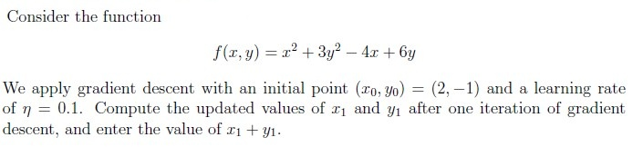
Gradient Descent
- Update rule:

x_{k+1} = x_k - \eta \nabla f(x_k)

Example: For $f(x,y) = x^2 + 3y^2 -4x +6y$ , compute:

\nabla f = (2x -4, 6y +6)

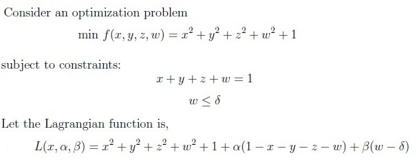
Karush-Kuhn-Tucker (KKT) Conditions
- For optimization with constraints:

\min f(x) \quad \text{s.t.} \quad h(x) = 0, \quad g(x) \leq 0

KKT Conditions:
1. Stationarity: $\nabla f(x) + \sum \alpha_i \nabla h_i(x) + \sum \beta_j \nabla g_j(x) = 0$ .
2. Primal feasibility: $h(x) = 0$ , $g(x) \leq 0$ .
3. Dual feasibility: $\beta_j \geq 0$ .
4. Complementary slackness: $\beta_j g_j(x) = 0$ .

D. Principal Component Analysis (PCA)

Key Ideas:
- Projects data onto directions of maximum variance (eigenvectors of covariance matrix).
- Principal components are uncorrelated and form an orthogonal basis.
- Steps:
  1. Compute covariance matrix $\Sigma$ .
  2. Find eigenvalues $\lambda_i$ and eigenvectors $v_i$ .
  3. Sort eigenvectors by descending $\lambda_i$ .

E. Function Analysis

Polynomial Functions
- Degree, roots, symmetry (even/odd), convexity.
- Example: $f(x) = x^4 -4x^2 +5$ :
  - Degree 4, no real roots (discriminant $< 0$ ), symmetric about y-axis, always non-negative.

Critical Points & Extrema
- Find critical points by setting $f'(x) = 0$ .
- Second derivative test for convexity/concavity.

2. Key Equations Summary

Topic	Equation
Joint PDF Transformation	$f_{U,V}(u,v) = f_{X,Y}(x,y) \cdot \|J\|^{-1}$
Expected Value	$E[aX + bY] = aE[X] + bE[Y]$
Markov’s Inequality	$P(X \geq a) \leq \frac{E[X]}{a}$
SVD	$A = U \Sigma V^T$ , $\sigma_i = \sqrt{\lambda_i(A^T A)}$
Gradient Descent	$x_{k+1} = x_k - \eta \nabla f(x_k)$
KKT Conditions	$\nabla L = 0$ , $\beta_j g_j(x) = 0$ , $\beta_j \geq 0$
PCA	$\Sigma v_i = \lambda_i v_i$ (eigenvalue problem)
Convex Function	$f(\lambda x + (1-\lambda)y) \leq \lambda f(x) + (1-\lambda)f(y)$

Graph 2: Linear Algebra & Optimization

Graph 3: Machine Learning (PCA)

Graph 4: Function Analysis

4. Exam Tips

Probability:
- Practice transforming joint PDFs using Jacobians.
- Memorize expected values for common distributions.

Linear Algebra:
- Understand SVD’s relationship with eigenvalues/eigenvectors.
- Know how to compute singular values from $A^T A$ .

Optimization:
- For KKT, focus on stationarity, primal/dual feasibility, and complementary slackness.
- Verify convexity before applying gradient descent.

PCA:
- Remember that principal components are uncorrelated and orthogonal.

Function Analysis:
- Check symmetry (even/odd), convexity (second derivative), and roots (discriminant).