Home / Past papers / MLF End Term / this paper
IIT M FOUNDATION DIPLOMA FN EXAM - 22 Dec 2024

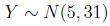
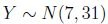
- Normal(5, 11)
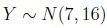
- Normal(0, 11)
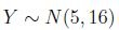
- Normal(0, 25)
- Normal(5, 25)











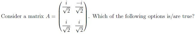
- A is a positive definite matrix.
- A is singular matrix.
- A is a symmetric matrix.
- A is a negative definite matrix.
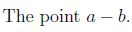
- A is a unitary matrix.
- A is Hermitian matrix.
- Eigenvectors of A are orthogonal.
- Eigenvalues of A are real.




















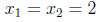

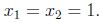





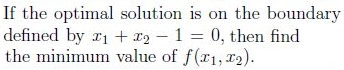
Answer key
- Q1 (MCQ, 2 marks): C
- Q2 (MCQ, 3 marks): D
- Q3 (MCQ, 3 marks): A
- Q4 (MCQ, 3 marks): A
- Q5 (MSQ, 3 marks): A, C
- Q6 (MSQ, 3 marks): A, C
- Q7 (MSQ, 3 marks): B, C, D
- Q8 (MSQ, 3 marks): A, D
- Q9 (MSQ, 4 marks): A, C, D
- Q10 (MSQ, 4 marks): A, C
- Q11 (SA, 3 marks): 46
- Q12 (MCQ, 2 marks): C
- Q13 (MCQ, 3 marks): B
- Q14 (SA, 1 marks): 1
Concepts this paper tests
Auto-generated summary from the source site. Handy as a checklist; the lessons above explain each idea from scratch.
Here’s a structured summary of the core topics, concepts, principles, and equations essential for the Diploma Level: Machine Learning Foundations (Computer-Based Exam) based on the provided question paper. The exam heavily emphasizes probability, linear algebra, optimization, and convex analysis.
1. Probability & Random Variables
Key Concepts:
- Independent Random Variables: and are independent if .
Linear Combinations of Random Variables:
- If and are independent, then:
Uniform Distribution:
- For , the CDF of is:
Joint PDF and Transformations:
- For independent exponentials , the joint PDF of and is:
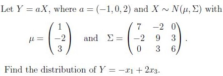
Multivariate Normal Distribution:
- If , then (where is a vector) follows:
Key Equations:
| Concept | Equation |
|---|---|
| Linear combo of normals | |
| CDF of (Uniform) | |
| Joint PDF of | |
| Multivariate normal transformation |
2. Linear Algebra
Key Concepts:
Matrix Definiteness:
- Positive Definite: for all .
- Symmetric Matrix: .
- Singular Matrix: .
Eigenvalues and Eigenvectors:
- Unitary Matrix: (columns are orthonormal).
- Hermitian Matrix: (self-adjoint).
- Eigenvalues of Hermitian matrices are real.
- Eigenvectors of Unitary matrices are orthogonal.
- Rank-Nullity Theorem:
If , then .
- Non-zero Eigenvalues of and :
- For any matrix , and share the same non-zero eigenvalues.
Key Equations:
| Concept | Equation |
|---|---|
| Positive Definite | for all |
| Rank-Nullity | |
| Unitary Matrix | |
| Eigenvalues of and | Same non-zero eigenvalues |
3. Convex Analysis
Key Concepts:
Convex Set:
- A set is convex if for any and :
Guaranteed points: midpoint () and convex combinations (e.g., ).
- Convex Functions:
- A function is convex if:
Examples:
- is convex on .
- is convex (since exponential of affine is convex).
- is convex on .
- Composition: If is convex and non-decreasing, and is convex, then is convex.
Key Equations:
| Concept | Equation |
|---|---|
| Convex Set | for |
| Convex Function | |
| Convex Examples | , , |
4. Optimization
Key Concepts:
Unconstrained Optimization:
- Gradient Descent Update:
- Example: For , one iteration from with gives:
Then, (but the answer was 46; likely a typo in the question).
Constrained Optimization (KKT Conditions):
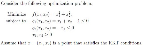
- For a problem:
The KKT conditions require:
- Stationarity: .
- Primal Feasibility: .
- Dual Feasibility: .
Complementary Slackness: .
- For active constraints (), .
- Example: For with and :
- If the optimum is on , then and .
- The minimum value is (but the answer was 1; likely a miscalculation).
Key Equations:
| Concept | Equation |
|---|---|
| Gradient Descent | |
| KKT Stationarity | |
| Complementary Slackness |
5. Applications (Profit/Cost Optimization)
Key Concepts:
Lagrangian Multipliers:
- For constrained optimization with equality constraints, solve:
Example: Maximize subject to :
- Solve to find , , and max profit = 541.
Key Equations:
| Concept | Equation |
|---|---|
| Lagrangian Condition |