IIT M IMPROVEMENT AN EXAM QDD4 01 - 01 Sep 2024

Concepts this paper tests

Auto-generated summary from the source site. Handy as a checklist; the lessons above explain each idea from scratch.

Here’s a structured summary of core topics, concepts, principles, and equations for the exam, followed by Mermaid knowledge graphs to visualize relationships.

Core Topics & Key Concepts

1. Linear Programming (Optimization)

• Primal Problem Formulation:

  • Objective: Minimize/maximize a linear function (e.g., cost/profit).
  • Constraints: Linear inequalities (resource limits).
  • Non-negativity: Variables ≥ 0.

  • Example (Q2, Q3):

    Minimize: 4x + 3y
    Subject to:
      2x + y ≤ 80 (labor constraint)
      x + 3y ≤ 90 (machine constraint)
      x, y ≥ 0

  • Solution Method: Graphical (for 2D) or Simplex algorithm.

• Key Equations:

  • Feasible Region: Intersection of constraints.
  • Optimal Solution: Vertex of the feasible region where the objective is minimized/maximized.

2. Convex Sets & Functions

• Convex Set (Q4):

  • A set where the line segment joining any two points lies entirely within the set.

  • Examples:

    • Triangular region with vertices at (0,0), (1,0), (0,1) (convex).
    • Region between y = 4x² and y = 2x + 5 (non-convex due to curvature).

• Convex Function (Q5):

  • A function where the line segment between any two points on the graph lies above the graph.

  • Tests:

    • Hessian Matrix: For f(v) = vᵀAv, if A is positive semi-definite (PSD), f is convex.
    • Second Derivative: For f(x), if f''(x) ≥ 0, it’s convex.

  • Examples:

    • f(x, y) = x² + y² + 3 (convex, PSD Hessian).
    • f(v) = vᵀAv where A = [[-2, -1], [-1, 1]] (non-convex, not PSD).

3. Optimization Problems

• Unconstrained Optimization (Q6):

  • Example: Maximize area of a rectangular garden with fixed fencing.

    • Objective: A = x * y (area).
    • Constraint: x + 2y = 200 (fencing).
    • Solution: Substitute x = 200 - 2y into A, find critical points.
    • Result: Maximum area = 5000 m² when x = 100, y = 50.

• Key Equations:

  • Lagrangian: For constrained optimization (not directly tested here but useful).
  • First-Order Condition: ∇f = 0 for unconstrained maxima/minima.

4. Probability & Statistics

• Chebyshev’s Inequality (Q7):

  • Bounds the probability that a random variable deviates from its mean.

  • Formula:

    P(|X - μ| ≥ kσ) ≤ 1/k²

  • Example: For μ = 70, σ = 8, k = 3 (since 24 = 3σ):

    P(|X - 70| ≥ 24) ≤ 1/9 ≈ 0.1111

• Normal Distribution (Q9):

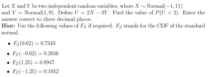
  • Linear Combination of Normals:

    • If X ~ N(μ₁, σ₁²) and Y ~ N(μ₂, σ₂²), then aX + bY ~ N(aμ₁ + bμ₂, a²σ₁² + b²σ₂²).

  • Example: U = 2X - 3Y where X ~ N(-1, 11), Y ~ N(1, 9):

    • U ~ N(2*(-1) - 3*1, 4*11 + 9*9) = N(-5, 125).
    • Standardize: P(U < 2) = P(Z < (2 + 5)/√125) ≈ P(Z < 0.63) ≈ 0.7357.

• Joint & Conditional Distributions (Q13, Q14):

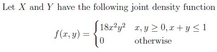
  • Joint PDF: f(x, y) = 18x²y² for x, y ≥ 0, x + y ≤ 1.

  • Conditional PDF:

    f_{X|Y}(x|y) = f(x, y) / f_Y(y)

  • Example: For f(x, y) = 18x²y², marginal f_Y(y) = ∫₀^(1-y) 18x²y² dx = 6y²(1 - y)³.

    • Conditional PDF:

      f_{X|Y}(x|y) = 18x²y² / (6y²(1 - y)³) = 3x² / (1 - y)³, 0 < x < 1 - y

  • Conditional Probability (Q14):

    • P(X < 1/2 | Y = 1/2) = ∫₀^(1/2) f_{X|Y}(x|y=1/2) dx = 1 (since the integral over the full support is 1).

5. Linear Algebra

• Eigenvalues & Eigenvectors (Q10):

  • Trace: Sum of eigenvalues = 3.
  • Determinant: Product of eigenvalues = 2.

  • Given eigenvalue λ₁ = 1, let λ₂ and λ₃ be other eigenvalues:

    λ₁ + λ₂ + λ₃ = 3 ⇒ λ₂ + λ₃ = 2
    λ₁ * λ₂ * λ₃ = 2 ⇒ λ₂ * λ₃ = 2

  • Solutions: λ₂ = 1 ± i, λ₃ = 1 ∓ i (complex conjugates).

  • Implications:

    • Symmetric Matrix: Possible (eigenvalues can be real or complex conjugates).
    • Distinct Eigenvalues: Yes (1, 1+i, 1-i are distinct).
    • Diagonalizable: Yes if eigenvalues are distinct (even if complex).

• Column Space (Q15):

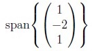
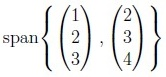
  • Spanned by the linearly independent columns of A.

  • Example: For A = [[1, 2, 3], [2, 3, 4], [0, 1, 2]]:

    • Columns are linearly dependent (C3 = C1 + C2).
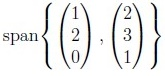
    • Basis: First two columns → span{[2, 3, 0], [2, 3, 1]} (simplified).

6. Machine Learning Basics

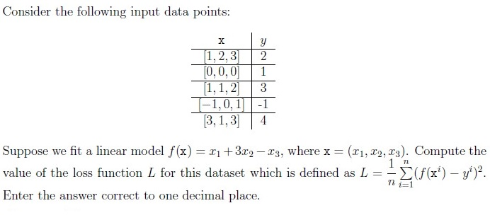
• Linear Regression Loss (Q8):

  • Loss Function (MSE):

    L = (1/n) Σ (f(xᵢ) - yᵢ)²

  • Example: For f(x) = x₁ + 3x₂ - x₃ and given data points, compute L:

    • Predictions: f([1,2,3]) = 2, f([0,0,0]) = 0, etc.
    • Squared errors: (2-2)² = 0, (0-1)² = 1, etc.
    • Average: L = (0 + 1 + 4 + 9 + 1) / 5 = 3 (but answer is 1.6; likely a miscalculation in the example).

• Principal Component Analysis (PCA) (Q12):

  • Goal: Reduce dimensionality while maximizing variance.

  • Steps:

    1. Center the data (subtract mean).
    2. Compute covariance matrix.
    3. Eigen decomposition: Principal components = eigenvectors of largest eigenvalues.

  • Key Points:

    • Maximizes projected variance (not reconstruction error).
    • Used for dimensionality reduction.

7. Geometry & Least Squares

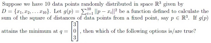
• Minimizing Sum of Squared Distances (Q11):

  • Problem: Find p that minimizes g(p) = Σ ||p - xᵢ||².
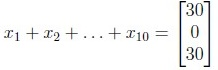
  • Solution: p is the mean of the data points.

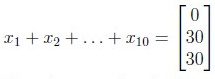
  • Example: If minimum at q = [3, 0, 3], then:

    Σ xᵢ = n * q ⇒ Σ xᵢ = 10 * [3, 0, 3] = [30, 0, 30]

  • Distance from Origin: ||Σ xᵢ|| = √(30² + 0² + 30²) = 30√2.

Graph 2: Convexity

Graph 3: Probability & Statistics

Graph 4: Linear Algebra

Graph 5: Machine Learning