ML Study Hub

Home / Past papers / MLF End Term / this paper

IIT M FOUNDATION DIPLOMA FN EXAM QDF1 28 Apr 2024 - 28 Apr 2024

MLF End Term14 questions40 marks6 MSQ · 6 SA · 2 MCQFoundation / Diploma / forenoon / QDF1
Elapsed 00:00
Comprehension passage - the questions below it refer to this
A person went to the market to buy hens. Old hens can be bought for ₹ 200.00 each but young hens can be bought for ₹ 500.00 each. The old hens lay 3 eggs per week and the young hens lay 5 eggs per week. Each egg costs Rs. 11. A hen costs ₹ 50.00 per week to feed. If the financial constraint is ₹ 8000 per week to buy hens and the capacity constraint is that the total number of hens bought cannot exceed 20 per week. The objective is to earn more profit. Let x represent the number of old hens and y represent the number of young hens. Use the above information to answer the given subquestions
Q1MCQ2 marks
Choose the correct Primal optimization problem from the following.
  1. question figure
  2. question figure
  3. question figure
  4. question figure
Q2MSQ2 marksselect all that apply
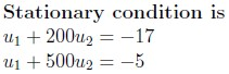
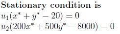
If (x*, y*) is the optimal solution of the primal, u1 and u2 are Lagrange multipliers then which of the following options is/are true?
  1. question figure
  2. question figure
  3. question figure
  4. question figure
  5. question figure
Q3MSQ3 marksselect all that apply
Which of the following options is/are true?
  1. The Given LPP is infeasible.
  2. The Given LPP is feasible.
  3. The optimum value is x = 0 and y = 16
  4. The optimum value is x = 20 and y = 0
Q4SA3 marks
question figure
Q5MSQ3 marksselect all that apply
question figure
  1. question figure
  2. question figure
  3. question figure
  4. question figure
Q6MSQ3 marksselect all that apply
question figure
  1. question figure
  2. question figure
  3. question figure
  4. question figure
Comprehension passage - the questions below it refer to this
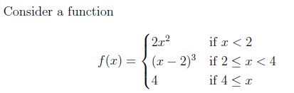
Based on the above data, answer the given subquestions. question figure
Q7SA3 marks
Find the number of discontinuous points.
Q8SA3 marks
Find the number of points where the function is not differentiable.
Q9MSQ3 marksselect all that apply
Let A be a real symmetric positive definite matrix. Which of the following options is/are true?
  1. The eigenvectors of A may or may not be orthogonal.
  2. If A is similar to a diagonal matrix B, then B is also positive definite.
  3. AT A is not positive definite.
  4. AT A is not similar to a diagonal matrix.
Q10MSQ3 marksselect all that apply
question figure
  1. question figure
  2. question figure
  3. question figure
  4. question figure
Q11MCQ3 marks
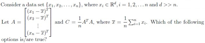
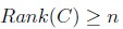
question figure
  1. question figure
  2. question figure
  3. question figure
  4. question figure
Q12SA3 marks
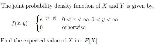
question figure
Q13SA3 marks
In a large town, it is estimated that 20% of students own a laptop. A random sample of 400 students is selected from the town. What is the variance of the number of students with the laptops in a given sample?
Q14SA3 marks
A quality control manager at a factory measures the thickness of glass sheets produced. Five randomly selected sheets have the thicknesses(in mm) 10, 8, 11, 9, 12 respectively. Assuming the thickness follows a normal distribution and the variance is known, what is the maximum likelihood estimator (MLE) of the mean thickness, (μ), in mm of the glass sheets?

Answer key

  1. Q1 (MCQ, 2 marks): A
  2. Q2 (MSQ, 2 marks): C
  3. Q3 (MSQ, 3 marks): B, C
  4. Q4 (SA, 3 marks): 4
  5. Q5 (MSQ, 3 marks): A, C, D
  6. Q6 (MSQ, 3 marks): B, D
  7. Q7 (SA, 3 marks): 2
  8. Q8 (SA, 3 marks): 2
  9. Q9 (MSQ, 3 marks): A, B
  10. Q10 (MSQ, 3 marks): B, C
  11. Q11 (MCQ, 3 marks): A
  12. Q12 (SA, 3 marks): 1
  13. Q13 (SA, 3 marks): 64
  14. Q14 (SA, 3 marks): 10

Concepts this paper tests

Auto-generated summary from the source site. Handy as a checklist; the lessons above explain each idea from scratch.

Here’s a structured summary of core topics, concepts, principles, and equations essential for the exam, followed by Mermaid knowledge graphs to visualize relationships.


1. Core Topics & Key Concepts

A. Linear Programming (LP) & Optimization

Key Concepts:

  1. Primal Problem Formulation:

    • Objective: Maximize/Minimize a linear function (e.g., profit).
    • Constraints: Linear inequalities (e.g., budget, capacity).
    • Non-negativity: Variables ≥ 0.
    • Example (from Q2):

      • Maximize: 5y−17x5y - 17x (profit function derived from egg sales minus costs).
      • Subject to:
x+y≤20(capacity constraint),x + y \leq 20 \quad \text{(capacity constraint)},
200x+500y≤8000(budget constraint).200x + 500y \leq 8000 \quad \text{(budget constraint)}.
  1. Feasibility & Optimality:

    • Feasible Region: Set of points satisfying all constraints.
    • Optimal Solution: Vertex of the feasible region (use corner point method or simplex algorithm).
    • Example (from Q4): Optimal solution is x=0,y=16x = 0, y = 16.
  1. Lagrange Multipliers & KKT Conditions:

    • Complementary Slackness: For active constraints, multipliers ui≠0u_i \neq 0; else ui=0u_i = 0.
u1(x∗+y∗−20)=0,u2(200x∗+500y∗−8000)=0.u_1(x^* + y^* - 20) = 0, \quad u_2(200x^* + 500y^* - 8000) = 0.
∇f(x∗,y∗)+u1∇g1(x∗,y∗)+u2∇g2(x∗,y∗)=0.\nabla f(x^*, y^*) + u_1 \nabla g_1(x^*, y^*) + u_2 \nabla g_2(x^*, y^*) = 0.

Equations:


B. Convexity & Optimization

Key Concepts:

  1. Convex Functions:

    • Definition: f(λx+(1−λ)y)≤λf(x)+(1−λ)f(y)f(\lambda x + (1-\lambda)y) \leq \lambda f(x) + (1-\lambda)f(y) for λ∈[0,1]\lambda \in [0,1].
    • Examples (from Q6):

      • f(x,y)=2x2+3y2f(x, y) = 2x^2 + 3y^2 (convex, as Hessian is positive semi-definite).
      • g(x)=−(x+1)2g(x) = -(x + 1)^2 (concave, not convex).
  1. Convex Sets:

    • Definition: For any x,yx, y in the set, λx+(1−λ)y\lambda x + (1-\lambda)y is also in the set.
    • Examples (from Q7):

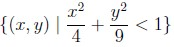
      • Convex: x2+y2<1x^2 + y^2 < 1 (interior of a circle), x24+y29<1\frac{x^2}{4} + \frac{y^2}{9} < 1 (interior of an ellipse).

      • Non-convex: x2+y2=1x^2 + y^2 = 1 (boundary), x2+y2>1x^2 + y^2 > 1 (exterior).
  1. Global vs. Local Minima:

    • For convex functions, any local minimum is a global minimum.

Equations:

Hf=[∂2f∂x2∂2f∂x∂y∂2f∂y∂x∂2f∂y2].H_f = \begin{bmatrix} \frac{\partial^2 f}{\partial x^2} & \frac{\partial^2 f}{\partial x \partial y} \\ \frac{\partial^2 f}{\partial y \partial x} & \frac{\partial^2 f}{\partial y^2} \end{bmatrix}.

C. Calculus & Function Analysis

Key Concepts:

  1. Continuity & Differentiability:

    • Discontinuity: Points where lim⁡x→cf(x)≠f(c)\lim_{x \to c} f(x) \neq f(c).
    • Non-differentiability: Corners (e.g., ∣x∣|x| at x=0x=0) or discontinuities.
    • Example (from Q8, Q9):

      • Function:
f(x)={2x2x<2(x−2)32≤x<44x≥4.f(x) = \begin{cases} 2x^2 & x < 2 \\ (x-2)^3 & 2 \leq x < 4 \\ 4 & x \geq 4 \end{cases}.
  1. Optimization with Constraints:

    • Method: Lagrange multipliers or substitution.
    • Example (from Q5):

      • Maximize f(x,y)=xyf(x, y) = xy subject to x28+y22=2\frac{x^2}{8} + \frac{y^2}{2} = 2.
      • Solution: Use substitution y=2(2−x28)y = \sqrt{2(2 - \frac{x^2}{8})}, then find critical points.

Equations:

L(x,y,λ)=f(x,y)−λg(x,y).\mathcal{L}(x, y, \lambda) = f(x, y) - \lambda g(x, y).

D. Linear Algebra

Key Concepts:

  1. Positive Definite Matrices:

    • Definition: xTAx>0x^T A x > 0 for all x≠0x \neq 0.
    • Properties (from Q10):

      • Eigenvalues > 0.
      • Eigenvectors are orthogonal.
      • ATAA^T A is positive definite if AA is invertible.
  1. Rank & PCA:

    • Rank: Maximum number of linearly independent rows/columns.
    • PCA (Principal Component Analysis):

      • For data matrix AA, compute covariance matrix C=1nATAC = \frac{1}{n} A^T A.
      • If d>>nd >> n, use 1nAAT\frac{1}{n} A A^T (from Q11).

Equations:

C=1nATA,A=[(x1−x‾)T⋮(xn−x‾)T].C = \frac{1}{n} A^T A, \quad A = \begin{bmatrix} (x_1 - \overline{x})^T \\ \vdots \\ (x_n - \overline{x})^T \end{bmatrix}.
C=VΛVT,Λ=diag(λ1,…,λd).C = V \Lambda V^T, \quad \Lambda = \text{diag}(\lambda_1, \dots, \lambda_d).

E. Probability & Statistics

Key Concepts:

  1. Exponential Distribution:

    • PDF: f(x)=λe−λxf(x) = \lambda e^{-\lambda x}.
    • Transformation of Variables (from Q12):

      • Given Y1=X1+X2Y_1 = X_1 + X_2, Y2=X1−X2Y_2 = X_1 - X_2, find joint PDF using Jacobian:
fY1,Y2(y1,y2)=fX1,X2(x1,x2)⋅∣J∣,f_{Y_1, Y_2}(y_1, y_2) = f_{X_1, X_2}(x_1, x_2) \cdot |J|,

where JJ is the Jacobian determinant.

  1. Expected Value:

    • For independent exponentials X∼Exp(λ)X \sim \text{Exp}(\lambda), E[X]=1λE[X] = \frac{1}{\lambda}.
    • Example (from Q13): E[X]=1E[X] = 1 for λ=1\lambda = 1.
  1. Binomial Distribution:

    • Variance: np(1−p)np(1-p).
    • Example (from Q14): n=400n = 400, p=0.2p = 0.2, variance = 400×0.2×0.8=64400 \times 0.2 \times 0.8 = 64.
  1. Maximum Likelihood Estimation (MLE):

    • For normal distribution, MLE of mean μ\mu is the sample mean.
    • Example (from Q15): μ^=10+8+11+9+125=10\hat{\mu} = \frac{10 + 8 + 11 + 9 + 12}{5} = 10.

Equations:

fY1,Y2(y1,y2)=λ1λ22e−λ1+λ22y1−λ1−λ22y2,y1±y2≥0.f_{Y_1, Y_2}(y_1, y_2) = \frac{\lambda_1 \lambda_2}{2} e^{-\frac{\lambda_1 + \lambda_2}{2} y_1 - \frac{\lambda_1 - \lambda_2}{2} y_2}, \quad y_1 \pm y_2 \geq 0.
Var(X)=np(1−p).\text{Var}(X) = np(1-p).
μ^=1n∑i=1nxi.\hat{\mu} = \frac{1}{n} \sum_{i=1}^n x_i.

Graph 2: Convexity & Function Analysis

Graph 3: Probability & Statistics

Graph 4: Linear Algebra & PCA