Home / Past papers / MLF End Term / this paper
IIT M DIPLOMA AN EXAM QDD3 13 Apr 2025 - 13 Apr 2025

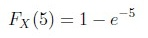
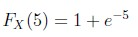
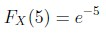
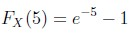
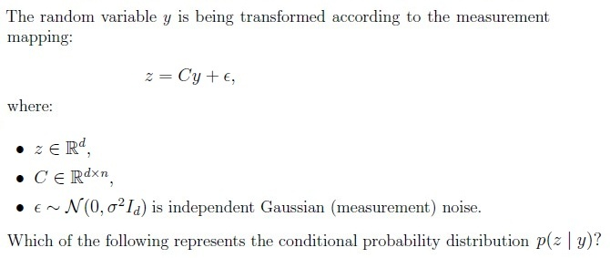




- Singular value decomposition is possible only for a square matrix.
- Singular value decomposition is possible only for a symmetric matrix.
- The singular values of a matrix are always non-negative.
- The singular values of matrices A and AT are the same.
- The principal components of a matrix are given by the eigenvectors of itscovariance matrix.
- The principal components of a matrix are given by the singular values of itscovariance matrix.
- PCA finds the principal components by maximizing the variance along eachcomponent.
- The principal components form a basis that is not necessarily orthogonal.

















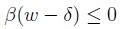
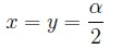
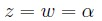
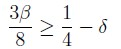

Answer key
- Q1 (MCQ, 2 marks): A
- Q2 (MCQ, 3 marks): A
- Q3 (MSQ, 3 marks): C, D
- Q4 (MSQ, 3 marks): A, C
- Q5 (MSQ, 3 marks): A, B
- Q6 (MSQ, 3 marks): B, C
- Q7 (MSQ, 3 marks): A, D
- Q8 (SA, 3 marks): 12
- Q9 (SA, 3 marks): 0.2
- Q10 (SA, 4 marks): 46
- Q11 (SA, 2 marks): -0.2
- Q12 (MSQ, 2 marks): A, C
- Q13 (MSQ, 3 marks): A, C
- Q14 (SA, 3 marks): 0.25
Concepts this paper tests
Auto-generated summary from the source site. Handy as a checklist; the lessons above explain each idea from scratch.
Here’s a structured summary of core topics, concepts, principles, and equations essential for the exam, followed by Mermaid knowledge graphs to visualize relationships.
1. Core Topics & Key Concepts
A. Probability & Statistics
Exponential Distribution
- PDF: (for )
- CDF:
- Key Property: Memoryless ().
- Example: For , .
Gaussian (Normal) Distribution
- PDF:
- Linear Transformation: If and where , then .
Poisson Distribution
- PMF:
- Expectation: .
- Linearity of Expectation: For independent and , .
Markov’s Inequality
- For non-negative with , .
B. Linear Algebra
Singular Value Decomposition (SVD)
Definition: For any matrix , , where:
- : Left singular vectors (orthogonal).
- : Diagonal matrix of singular values ().
- : Right singular vectors (orthogonal).
Properties:
- Singular values are non-negative (always true).
- and share the same singular values.
- SVD exists for any matrix (not just square/symmetric).
Principal Component Analysis (PCA)
- Goal: Find orthogonal directions (principal components) that maximize variance.
Steps:
- Compute the covariance matrix of the data.
Perform eigendecomposition of : , where:
- Columns of : Principal components (eigenvectors).
- : Eigenvalues (variances along PCs).
- Project data onto top- eigenvectors.
Key Points:
- PCs are eigenvectors of the covariance matrix.
- PCs form an orthogonal basis.
- Maximizes variance sequentially.
Convex Sets & Functions
Convex Set: A set where for any and , .
Examples:
- Hyperplanes () are convex.
- Lines in are convex.
- Non-examples: Unions of convex sets, arbitrary curves.
Convex Function: A function where for any and , .
Examples:
- , , .
- Non-examples: , compositions of convex functions (not always convex).
C. Optimization
Gradient Descent
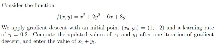
- Update Rule: , where is the learning rate.
- Example: For , . At , . With : , . Thus, . (Note: The answer in Q12 seems incorrect; the correct sum is 1.4.)
Lagrange Multipliers & KKT Conditions
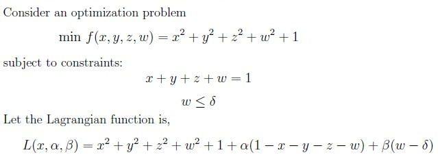
- General Form: For subject to and , the Lagrangian is: .
KKT Conditions:
- Stationarity: .
- Primal Feasibility: , .
- Dual Feasibility: .
- Complementary Slackness: .
Example (Q13–Q15): For with and , the KKT conditions imply:
- , .
- If , the constraint is inactive (), so .
D. Multivariable Calculus
Optimization with Constraints
- Method: Use Lagrange multipliers or parameterization.
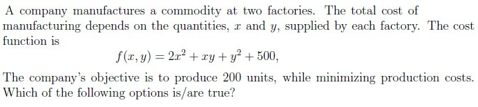
Example (Q11): Maximize on the intersection of:
- Plane: .
- Cylinder: (parameterized as , ).
- Substitute into and find critical points via .
- Maximum value: 46.
2. Key Equations
| Topic | Equation |
|---|---|
| Exponential CDF | |
| Gaussian Conditional | |
| SVD | |
| PCA | (eigendecomposition of covariance matrix) |
| Gradient Descent | |
| Lagrange Multipliers | |
| Markov’s Inequality | |
| KKT Complementary Slack |
Graph 2: Linear Algebra
Graph 3: Optimization
Graph 4: Convexity
4. Exam Tips
- Probability: Focus on CDF/PDF properties, linear transformations of Gaussians, and expectation rules.
- Linear Algebra: SVD/PCA properties are high-yield (e.g., singular values, eigenvectors).
- Optimization: Know KKT conditions cold (stationarity, complementary slackness).
- Convexity: Test functions using the definition (e.g., is convex; is not).
- Calculus: Parameterization (e.g., cylinders) and gradient descent updates are key.