Home / Past papers / MLF End Term / this paper
IIT M FOUNDATION FN EXAM FDF2 24 Dec 2023 - 24 Dec 2023
Elapsed 00:00
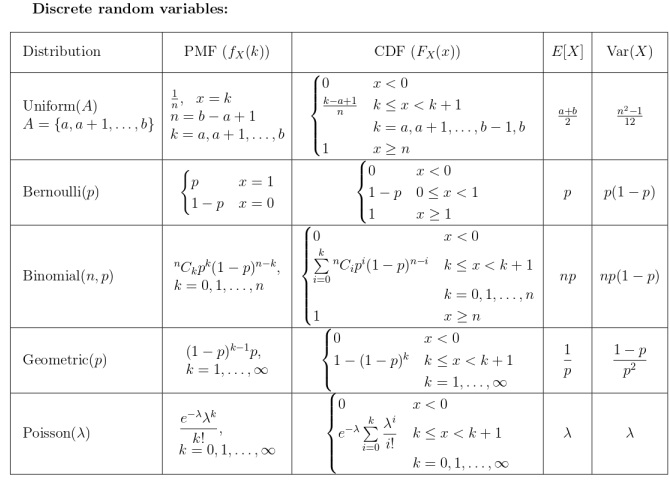
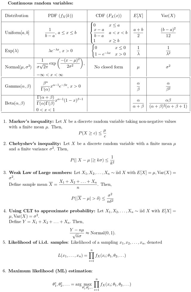
- Useful Data has been mentioned above.
- This data attachment is just for a reference & not for an evaluation.
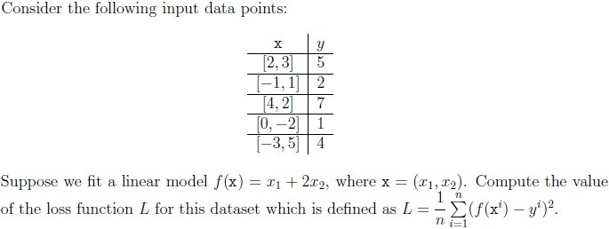
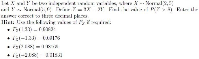


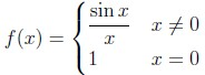
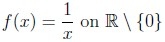
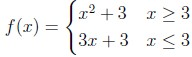
Which of the following functions is/are continuous?

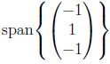
Let A be a n × n positive definite matrix. Then, which among the following are correct?



















Comprehension passage - the questions below it refer to this
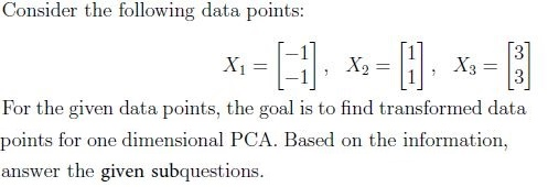
Which of the following represents the covariance matrix, C for the given data points?


What is the value of the projected variance? Enter the answer correct to two decimal places.

Answer key
- Q1 (MCQ, 0 marks): A
- Q2 (SA, 3 marks): 9
- Q3 (SA, 3 marks): 0.089 to 0.095
- Q4 (SA, 3 marks): 0.74 to 0.79
- Q5 (SA, 3 marks): 0.24 to 0.28
- Q6 (SA, 3 marks): 0.020 to 0.030
- Q7 (MSQ, 3 marks): A, B, D
- Q8 (MSQ, 3 marks): A, B, D
- Q9 (SA, 4 marks): 0.370 to 0.380
- Q10 (MSQ, 3 marks): B, C
- Q11 (MCQ, 2 marks): C
- Q12 (MCQ, 2 marks): B
- Q13 (MCQ, 2 marks): B
- Q14 (MCQ, 2 marks): C
- Q15 (SA, 2 marks): 5.30 to 5.37
- Q16 (SA, 2 marks): 10
Concepts this paper tests
Auto-generated summary from the source site. Handy as a checklist; the lessons above explain each idea from scratch.
Here’s a structured summary of core topics, concepts, principles, and equations essential for the exam, followed by Mermaid knowledge graphs to visualize relationships.
Core Topics & Concepts
1. Probability & Statistics
A. Random Variables & Distributions
Discrete Distributions:
- Uniform (Discrete): PMF, CDF, Mean (
(a+b)/2), Variance ((n²-1)/12). - Bernoulli: PMF, CDF, Mean (
p), Variance (p(1-p)). - Binomial: PMF (
nCk p^k (1-p)^(n-k)), Mean (np), Variance (np(1-p)). - Geometric: PMF (
(1-p)^(k-1) p), Mean (1/p), Variance ((1-p)/p²). - Poisson: PMF (
(e^-λ λ^k)/k!), Mean (λ), Variance (λ).
- Uniform (Discrete): PMF, CDF, Mean (
Continuous Distributions:
- Uniform (Continuous): PDF (
1/(b-a)), CDF, Mean ((a+b)/2), Variance ((b-a)²/12). - Exponential: PDF (
λe^-λx), CDF (1-e^-λx), Mean (1/λ), Variance (1/λ²). - Normal: PDF (
(1/σ√2π) e^(-(x-μ)²/2σ²)), Mean (μ), Variance (σ²). - Gamma: PDF (
(β^α/Γ(α)) x^(α-1) e^-βx), Mean (α/β), Variance (α/β²). - Beta: PDF (
Γ(α+β)/Γ(α)Γ(β) x^(α-1) (1-x)^(β-1)), Mean (α/(α+β)), Variance (αβ/((α+β)²(α+β+1))).
- Uniform (Continuous): PDF (
B. Inequalities & Theorems
- Markov’s Inequality:
P(X ≥ c) ≤ μ/c(for non-negativeX). - Chebyshev’s Inequality:
P(|X-μ| ≥ kσ) ≤ 1/k². - Weak Law of Large Numbers (WLLN):
P(|X̄ - μ| > δ) ≤ σ²/(nδ²)whereX̄ = (X₁ + ... + Xₙ)/n. - Central Limit Theorem (CLT):
(Y - nμ)/(σ√n) ≈ N(0,1)whereY = X₁ + ... + Xₙ.
C. Maximum Likelihood Estimation (MLE)
- Likelihood Function:
L(θ) = ∏ f_X(x_i; θ). - MLE Estimator:
θ* = argmax_θ L(θ).
D. Joint & Conditional Distributions
- Joint PDF/PMF:
f_X,Y(x,y). - Conditional Expectation:
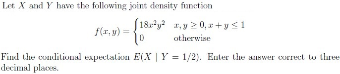
E[X|Y=y] = ∫ x f_X|Y(x|y) dx.
2. Linear Algebra
A. Matrix Properties
Positive Definite Matrices:
Ais positive definite ifxᵀAx > 0for allx ≠ 0.Properties:
A^kis positive definite fork ≥ 1.- Diagonal entries of
Aare positive. A⁻¹is positive definite.rAis positive definite forr > 0.
Eigenvalues & Eigenvectors:
Av = λv.det(A - λI) = 0(characteristic equation).- If
Ahasnlinearly independent eigenvectors, it is diagonalizable.
- Nullspace:
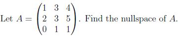
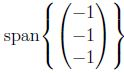
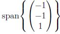
Null(A) = {x | Ax = 0}.
B. Optimization & Convexity
Convex Functions:
f(αx + (1-α)y) ≤ αf(x) + (1-α)f(y)forα ∈ [0,1].- Examples:
f(x) = 1/x(convex forx > 0),g(x) = 1 + |x|(convex). Composition rules:
g ∘ fis convex ifgis convex and non-decreasing, andfis convex.- Sum of convex functions is convex.
3. Machine Learning & Optimization
A. Linear Regression
- Loss Function (MSE):
L = (1/n) Σ (f(xᵢ) - yᵢ)²(forf(x) = w₁x₁ + w₂x₂ + ...). (Note: Question 3 usesL = - (1/n) Σ (f(xᵢ) - yᵢ)², which is negative MSE.)
B. Principal Component Analysis (PCA)
- Covariance Matrix:
C = (1/n) XᵀX(for centered data). - Projected Variance: Maximized along the principal component (eigenvector of
Cwith largest eigenvalue).
C. Linear Programming
Standard Form:
- Maximize
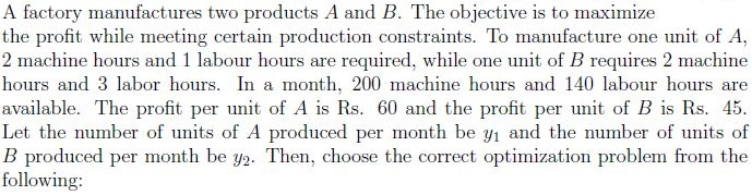
cᵀysubject toAy ≤ b,y ≥ 0. Example (Question 14):
Maximize Z = 60y₁ + 45y₂
Subject to:
  2y₁ + 2y₂ ≤ 200
  y₁ + 3y₂ ≤ 140
  y₁, y₂ ≥ 0
- Maximize
4. Calculus & Continuity
Continuous Functions:
lim_{x→a} f(x) = f(a).Examples:
sin(x)/x(continuous atx=0if defined as1).- Piecewise functions (e.g.,
x² + 3forx ≥ 3,3x + 3forx < 3).
5. Geometry & Optimization
Maximizing Area with Fixed Perimeter:
- For a rectangle with perimeter
P, the maximum area is achieved when it’s a square (side = P/4). - Example (Question 7):
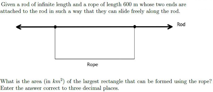
P = 600 ⇒ side = 150 ⇒ area = 22500.
- For a rectangle with perimeter
Constrained Optimization:
- Lagrange Multipliers: For
f(x,y)subject tog(x,y) = c, solve∇f = λ∇g. - Example (Question 17): Maximize
f(x,y) = x + ysubject tox² + y² = 50. Solution:x = y = 5⇒f(x,y) = 10.
- Lagrange Multipliers: For
Key Equations
| Topic | Equation | |||
|---|---|---|---|---|
| Markov’s Inequality | P(X ≥ c) ≤ μ/c | |||
| Chebyshev’s Inequality | `P( | X-μ | ≥ kσ) ≤ 1/k²` | |
| WLLN | `P( | X̄ - μ | > δ) ≤ σ²/(nδ²)` | |
| CLT | (Y - nμ)/(σ√n) ≈ N(0,1) | |||
| MLE | θ* = argmax_θ ∏ f_X(x_i; θ) | |||
| Conditional Expectation | `E[X | Y=y] = ∫ x f_X | Y(x | y) dx` |
| PCA Variance | Projected Variance = λ₁ (largest eigenvalue of covariance matrix) | |||
| Linear Regression Loss | L = (1/n) Σ (f(xᵢ) - yᵢ)² (or negative for Question 3) | |||
| Lagrange Multipliers | ∇f = λ∇g |