Home / Past papers / MLF End Term / this paper

IIT M FOUNDATION ET1 EXAM QPF1 S1 03 Sep - 03 Sep 2023

MLF End Term18 questions50 marks7 MSQ · 6 SA · 5 MCQFoundation / QPF1

Elapsed 00:00

Q1MCQ0 marks

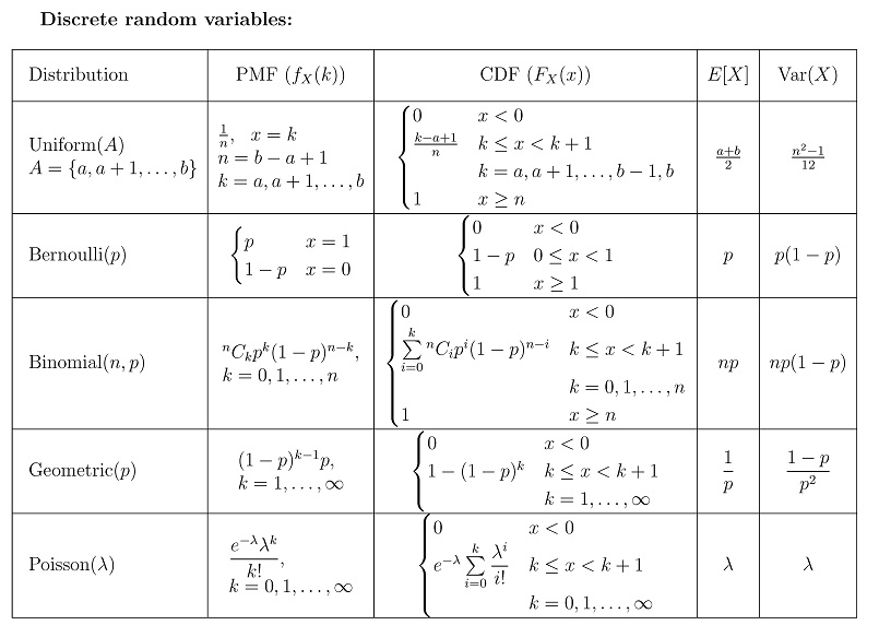
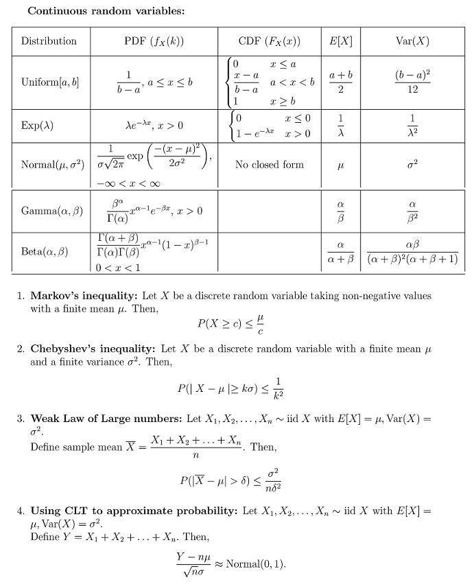
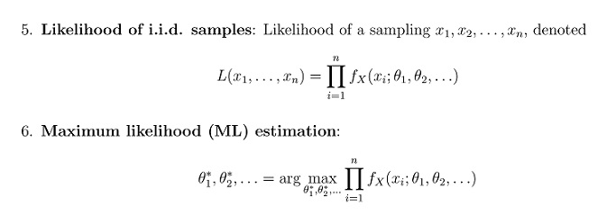
Useful Data has been mentioned above.
This data attachment is just for a reference & not for an evaluation.

Q2MSQ2 marksselect all that apply

Which of the following statements accurately describes the key difference between classification and regression models?

In classification, the output variable is continuous and real-valued, while inregression, it is categorical.
Regression models are used for predicting probabilities, whereas classificationmodels focus on predicting absolute values.
Classification models aim to find decision boundaries to separate data intoclasses, while regression models seek to predict a numeric value.
In regression, the commonly used loss function is mean squared error, whilein classification, 0 -1 loss is typically employed.

Comprehension passage - the questions below it refer to this

Based on the above data, answer the given subquestions. question figure

Q3SA2 marks

Your numeric answer:

Q4SA1 mark

Your numeric answer:

Q5MCQ3 marks

b1 − b2 + b3 = 0
b1 + b2 + b3 = 0
2b1 − b2 + b3 = 0
2b1 + b2 + b3 = 0

Q6MCQ3 marks

A consumer wants to maximize his utility subject to some constraints. He consumes two goods g1 and g2 and the utility function is the sum of g1 and g2. His budget is Rs.100. The per unit price of goods g1 and g2 are Rs.3 and Rs.4 respectively. Chose the correct optimization problem.

Q7MSQ4 marksselect all that apply

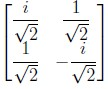
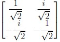
A − I (where I is the identity matrix of the same size) is also orthogonal.
Both AB and BA are orthogonal.
An and Bn are orthogonal for every n > 1.
A and B are also symmetric matrices.

Q8MSQ4 marksselect all that apply

Which of the following statements is/are true for a real symmetric matrix A?

AT A and AAT have the same rank.
AT A and AAT have the same eigenvalues
AT A and AAT have the same eigenvectors.
AT A and AAT have the same singular values.

Q9MSQ3 marksselect all that apply

Which of the following matrices is/are Unitary but not Hermitian?

Q10MSQ3 marksselect all that apply

Which among the following is true for PCA?

The first principal component represents the direction along which thevariance of the dataset is maximized.
The first principal component represents the direction along which thevariance of the dataset is minimized.
The first principal component is the eigenvector corresponding to the smallesteigenvalue of the covariance matrix.
The first principal component is the eigenvector corresponding to the largesteigenvalue of the covariance matrix.

Q11MSQ3 marksselect all that apply

Which of the following statements regarding gradient descent is/are correct?

If the step size is chosen as 1, we may “not always” arrive as close to theoptimal solution even after many number of iterations.
Solution obtained for optimization problem is the local minimum of itsobjective function.
Solution obtained for optimization problem is the global minimum of itsobjective function.
Gradient descent converges to the global optimum in the case of convexfunctions.
Gradient descent does not converge to the global optimum in the case ofconvex functions.

Q12MSQ3 marksselect all that apply

Suppose a fair coin is tossed twice. Let A denote the event that the first toss is a tail. Let B denote the event that the second toss is a tail. Let C denote the event that out of the first two tosses, either both are heads or both are tails. Which among the following options are true? Select all that apply.

A, B and C are independent.
A, B and C are dependent.
A, B and C are pairwise independent.
P(A) = P(B) = P(C) = 1/2

Q13SA2 marks

Your numeric answer:

Q14SA3 marks

Your numeric answer:

Q15SA3 marks

Your numeric answer:

Q16SA3 marks

The average life (in years) of an electric bulb follows exponential distribution with parameter λ = 0.4. Using Weak Law of large numbers, find a lower bound on the probability that the mean life of a random sample of 50 such bulbs falls between 1.5 and 3.5 years. Enter your answer correct to three decimal places.

Your numeric answer:

Q17MCQ4 marks

Q18MCQ4 marks

Answer key

Q1 (MCQ, 0 marks): A
Q2 (MSQ, 2 marks): C, D
Q3 (SA, 2 marks): 0
Q4 (SA, 1 marks): 7.44 to 7.52
Q5 (MCQ, 3 marks): C
Q6 (MCQ, 3 marks): A
Q7 (MSQ, 4 marks): B, C
Q8 (MSQ, 4 marks): A, B, D
Q9 (MSQ, 3 marks): A, D
Q10 (MSQ, 3 marks): A, D
Q11 (MSQ, 3 marks): A, B, D
Q12 (MSQ, 3 marks): B, C, D
Q13 (SA, 2 marks): 225
Q14 (SA, 3 marks): 1
Q15 (SA, 3 marks): 40
Q16 (SA, 3 marks): 0.870 to 0.880
Q17 (MCQ, 4 marks): C
Q18 (MCQ, 4 marks): A

Concepts this paper tests

Auto-generated summary from the source site. Handy as a checklist; the lessons above explain each idea from scratch.

Here’s a structured summary of core topics, concepts, principles, and equations for the exam, followed by Mermaid knowledge graphs to visualize relationships.

Core Topics & Concepts

1. Probability & Statistics

Key Distributions (Discrete & Continuous)

Distribution	PMF/PDF	CDF	Mean ( $E[X]$ )	Variance ( $\text{Var}(X)$ )
Uniform (Discrete)	$f_X(k) = \frac{1}{n}, \quad k = a, a+1, \dots, b$	$F_X(x) = \frac{k-a+1}{n}, \quad a \leq x < b$	$\frac{a+b}{2}$	$\frac{n^2-1}{12}$
Bernoulli	$f_X(k) = p^k (1-p)^{1-k}, \quad k=0,1$	$F_X(x) = 1-p, \quad 0 \leq x < 1$	$p$	$p(1-p)$
Binomial	$f_X(k) = {}^nC_k p^k (1-p)^{n-k}, \quad k=0,1,\dots,n$	$F_X(x) = \sum_{i=0}^k {}^nC_i p^i (1-p)^{n-i}$	$np$	$np(1-p)$
Geometric	$f_X(k) = (1-p)^{k-1}p, \quad k=1,2,\dots$	$F_X(x) = 1-(1-p)^k$	$\frac{1}{p}$	$\frac{1-p}{p^2}$
Poisson	$f_X(k) = \frac{e^{-\lambda} \lambda^k}{k!}, \quad k=0,1,\dots$	$F_X(x) = e^{-\lambda} \sum_{i=0}^k \frac{\lambda^i}{i!}$	$\lambda$	$\lambda$
Uniform (Continuous)	$f_X(x) = \frac{1}{b-a}, \quad a \leq x \leq b$	$F_X(x) = \frac{x-a}{b-a}$	$\frac{a+b}{2}$	$\frac{(b-a)^2}{12}$
Exponential	$f_X(x) = \lambda e^{-\lambda x}, \quad x \geq 0$	$F_X(x) = 1-e^{-\lambda x}$	$\frac{1}{\lambda}$	$\frac{1}{\lambda^2}$
Normal	$f_X(x) = \frac{1}{\sigma \sqrt{2\pi}} e^{-\frac{(x-\mu)^2}{2\sigma^2}}$	No closed form	$\mu$	$\sigma^2$
Gamma	$f_X(x) = \frac{\beta^\alpha}{\Gamma(\alpha)} x^{\alpha-1} e^{-\beta x}$	-	$\frac{\alpha}{\beta}$	$\frac{\alpha}{\beta^2}$
Beta	$f_X(x) = \frac{\Gamma(\alpha+\beta)}{\Gamma(\alpha)\Gamma(\beta)} x^{\alpha-1} (1-x)^{\beta-1}$	-	$\frac{\alpha}{\alpha+\beta}$	$\frac{\alpha\beta}{(\alpha+\beta)^2(\alpha+\beta+1)}$

Key Theorems & Inequalities

Markov’s Inequality:

P(X \geq c) \leq \frac{E[X]}{c}, \quad c > 0

Chebyshev’s Inequality:

P(|X - \mu| \geq k\sigma) \leq \frac{1}{k^2}

Weak Law of Large Numbers (WLLN):

P(|\overline{X} - \mu| > \delta) \leq \frac{\sigma^2}{n\delta^2}

Central Limit Theorem (CLT):

\frac{Y - n\mu}{\sqrt{n\sigma}} \approx \text{Normal}(0,1)

where $Y = X_1 + X_2 + \dots + X_n$ .

Maximum Likelihood Estimation (MLE):

\theta^* = \arg \max_\theta \prod_{i=1}^n f_X(x_i; \theta)

2. Linear Algebra

Key Concepts

Orthogonal Matrices:
- $A^T A = I$
- $AB$ is orthogonal if $A, B$ are orthogonal.
- $A + B$ is not necessarily orthogonal.
Symmetric Matrices:
- $A = A^T$
- Eigenvalues are real.
- $A^T A$ and $AA^T$ have the same eigenvalues and singular values (but not necessarily eigenvectors).
Unitary Matrices:
- $U^\dagger U = I$ (for complex matrices).
- Not necessarily Hermitian (e.g., rotation matrices).
Rank & Eigenvalues:
- $A^T A$ and $AA^T$ have the same rank.
Singular Value Decomposition (SVD):
- $A = U \Sigma V^T$ , where $\Sigma$ contains singular values.

Key Equations

Condition for Solvability of $A\mathbf{x} = \mathbf{b}$ :
- For $A \in \mathbb{R}^{m \times n}$ , $\mathbf{b}$ must lie in the column space of $A$ .
- Example: For the given matrix $A$ , the condition was $2b_1 - b_2 + b_3 = 0$ .

Distance from Origin to Surface:
- For $x^2 - y^2 - z^2 = 1$ , the minimum distance is 1 (using Lagrange multipliers or geometric intuition).

3. Optimization & Gradient Descent

Key Concepts

Gradient Descent:
- Update rule: $\mathbf{x}^{(k+1)} = \mathbf{x}^{(k)} - \alpha \nabla f(\mathbf{x}^{(k)})$ .
- Convergence:
  - Guaranteed to global minimum for convex functions.
  - May converge to local minima otherwise.
- Step Size ( $\alpha$ ):
  - If $\alpha$ is too large, it may diverge.
  - If $\alpha$ is too small, it may converge slowly.
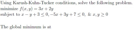
Karush-Kuhn-Tucker (KKT) Conditions:
- Necessary for optimality in constrained optimization.
- Conditions:
  1. Stationarity: $\nabla f(x^*) + \sum \lambda_i \nabla g_i(x^*) = 0$ .
  2. Primal Feasibility: $g_i(x^*) \leq 0$ .
  3. Dual Feasibility: $\lambda_i \geq 0$ .
  4. Complementary Slackness: $\lambda_i g_i(x^*) = 0$ .

Key Equations

Gradient of Quadratic Function:
- For $f(x_1, x_2) = 8x_1^2 + 2x_1x_2 - x_2^2$ :

\nabla f = (16x_1 + 2x_2, 2x_1 - 2x_2)

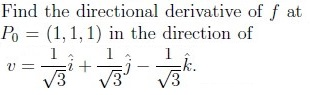
Directional Derivative:
- $D_{\mathbf{v}} f(\mathbf{x}) = \nabla f(\mathbf{x}) \cdot \mathbf{v}$ .
- Maximum rate of change: $\|\nabla f\|$ .

4. Machine Learning Foundations

Key Concepts

Classification vs. Regression: | Aspect | Classification | Regression | |---------------------|--------------------------------------------|----------------------------------------| | Output | Categorical (discrete) | Continuous (real-valued) | | Goal | Find decision boundaries | Predict numeric values | | Loss Function | 0-1 Loss, Cross-Entropy | Mean Squared Error (MSE) |

Principal Component Analysis (PCA):
- First PC: Direction of maximum variance (eigenvector of covariance matrix with largest eigenvalue).
- Subsequent PCs: Orthogonal directions with decreasing variance.

Independence of Random Variables:
- $X_1, X_2$ are independent iff $f_{X_1,X_2}(x_1,x_2) = f_{X_1}(x_1) f_{X_2}(x_2)$ .
- For Gaussian variables, uncorrelatedness implies independence.

Key Equations

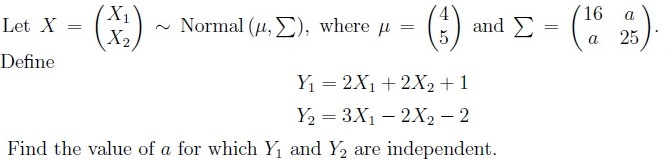
Transformation of Gaussian Variables:
- If $\mathbf{X} \sim \text{Normal}(\mu, \Sigma)$ , then $\mathbf{Y} = A\mathbf{X} + \mathbf{b} \sim \text{Normal}(A\mu + \mathbf{b}, A\Sigma A^T)$ .
- Independence Condition: For $Y_1 = 2X_1 + 2X_2 + 1$ and $Y_2 = 3X_1 - 2X_2 - 2$ , $Y_1$ and $Y_2$ are independent if $\text{Cov}(Y_1, Y_2) = 0$ .
  - Computed as $a = 40$ in the given problem.

Exponential Distribution:
- $X \sim \text{Exp}(\lambda)$ , $E[X] = \frac{1}{\lambda}$ , $\text{Var}(X) = \frac{1}{\lambda^2}$ .
- Weak Law of Large Numbers (WLLN) Application:
  - For $\lambda = 0.4$ , $E[X] = 2.5$ .
  - For $n = 50$ , $P(1.5 \leq \overline{X} \leq 3.5) \geq 0.875$ (using Chebyshev’s inequality).

5. Multivariable Calculus

Key Concepts

Gradient ( $\nabla f$ ):
- Points in the direction of steepest ascent.
- Magnitude $\|\nabla f\|$ gives the maximum rate of change.
Directional Derivative:
- $D_{\mathbf{v}} f = \nabla f \cdot \mathbf{v}$ .
Optimization with Constraints:
- Lagrange Multipliers: Used to find extrema of $f(x,y,z)$ subject to $g(x,y,z) = 0$ .

Key Equations

Gradient of $f(x,y,z) = x^2 + 2y^2 - 3z^2$ :

\nabla f = (2x, 4y, -6z)

Directional Derivative at $P_0 = (1,1,1)$ in direction $\mathbf{v}$ :

D_{\mathbf{v}} f = \nabla f(P_0) \cdot \mathbf{v} = (2,4,-6) \cdot \left( -\frac{1}{\sqrt{3}}, \frac{1}{\sqrt{3}}, -\frac{1}{\sqrt{3}} \right) = 0

Maximum Rate of Change at $P_0$ :

\|\nabla f(P_0)\| = \sqrt{2^2 + 4^2 + (-6)^2} = \sqrt{4 + 16 + 36} = \sqrt{56} \approx 7.48

IIT M FOUNDATION ET1 EXAM QPF1 S1 03 Sep - 03 Sep 2023

Answer key

Concepts this paper tests

Core Topics & Concepts

1. Probability & Statistics

Key Distributions (Discrete & Continuous)

Key Theorems & Inequalities

2. Linear Algebra

Key Concepts

Key Equations

3. Optimization & Gradient Descent

Key Concepts

Key Equations

4. Machine Learning Foundations

Key Concepts

Key Equations

5. Multivariable Calculus

Key Concepts

Key Equations

Graph 2: Linear Algebra

Graph 3: Optimization

Graph 4: Machine Learning

Graph 5: Multivariable Calculus