Home / Past papers / MLF End Term / this paper
IIT M FOUNDATION AN EXAM QDF3 31 Aug - 31 Aug 2025





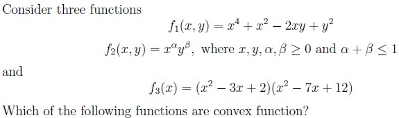









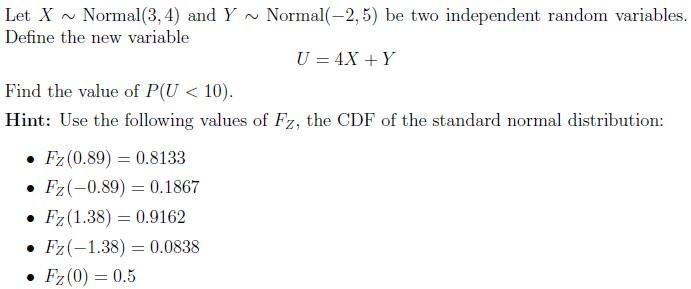










- S is a convex set.
- The objective function of the Primal optimization problem part (A) is a convexfunction.
- The objective function of the Primal optimization problem part (A) is a concavefunction.
- None of these
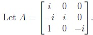

- A is not a Hermitian matrix.
- A is not a unitary matrix.
- A is diagonalizable.
- None of these
Answer key
- Q1 (MCQ, 3 marks): A
- Q2 (MSQ, 4 marks): A, C
- Q3 (MSQ, 3 marks): A, D
- Q4 (SA, 4 marks): 24
- Q5 (SA, 4 marks): 0.31 to 0.37
- Q6 (SA, 4 marks): 0.02 to 0.06
- Q7 (SA, 3 marks): 0.5
- Q8 (MCQ, 2 marks): B
- Q9 (MSQ, 2 marks): B, C
- Q10 (SA, 3 marks): 7.8
- Q11 (MSQ, 2 marks): A, B
- Q12 (SA, 3 marks): -125
- Q13 (MSQ, 3 marks): A, B
Concepts this paper tests
Auto-generated summary from the source site. Handy as a checklist; the lessons above explain each idea from scratch.
Here’s a structured summary of the core topics, concepts, principles, and equations essential for the Diploma Level: Machine Learning Foundations (Computer-Based Exam) based on the provided question paper. The exam covers probability, linear algebra, optimization, convexity, and statistics, with a focus on foundational mathematics for machine learning.
1. Core Topics & Key Concepts
A. Probability & Random Variables
Probability Inequalities
- Markov’s Inequality: For a non-negative random variable and :
Used for bounding tail probabilities (e.g., for ).
- Chebyshev’s Inequality:
For any random variable with mean , variance , and :
- Bounds deviation from the mean (e.g., ).
Binomial Distribution
:
- Mean:
- Variance:
Normal Distribution & Linear Combinations
- If and are independent, then:
- Standardization: .
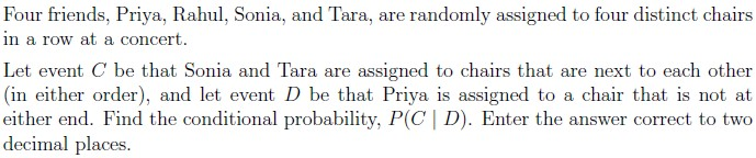
Conditional Probability
- Definition:
- Example: Permutations with constraints (e.g., seating arrangements).
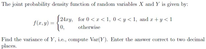
Joint Probability Density Functions (PDFs)
- For continuous random variables and , the joint PDF satisfies:
- Marginal PDF:
- Variance:
B. Linear Algebra
Vector Spaces & Span
- Span of a vector :
- Projection of onto :
- Orthogonality:
Eigenvalues & Eigenvectors
- For a matrix , eigenvalues satisfy .
Properties:
- Trace
- Determinant
- Diagonalizable Matrices: , where is diagonal.
- Hermitian Matrices: (equal to its conjugate transpose).
- Unitary Matrices: .
Matrix Operations
- Example: For with eigenvalues , the eigenvalues of are .
C. Optimization & Convexity
Convex Functions
- Definition: A function is convex if for all and :
Examples:
- (convex, as its Hessian is positive semidefinite).
- is convex on .
- Non-Convex Example: with is not convex in general.
Convex Sets
- Definition: A set is convex if for all and :
- Example: The set is convex.
Optimization Problems
- Primal Problem: Minimize a convex objective subject to convex constraints. Example:
- Lagrangian Function:
- Stationary Conditions (KKT Conditions):
D. Calculus & Quadratic Forms
Hessian Matrix
- For a function , the Hessian is:
- Convexity Test: is convex if is positive semidefinite.
Quadratic Optimization
- Example: Minimizing subject to .
- Solution: Use substitution and calculus to find critical points.
2. Key Equations Summary
| Topic | Equation |
|---|---|
| Markov’s Inequality | |
| Chebyshev’s Inequality | |
| Binomial Mean/Variance | , |
| Normal Linear Combination | |
| Projection | |
| Conditional Probability | |
| Joint PDF Marginalization | |
| Variance | |
| Eigenvalues of | , where are eigenvalues of |
| Lagrangian | |
| KKT Conditions | , , |
| Hessian Convexity | (positive semidefinite) |
Graph 2: Linear Algebra
Graph 3: Optimization & Convexity
Graph 4: Relationships Between Topics
4. Exam Preparation Tips
Probability Inequalities:
- Practice applying Markov’s and Chebyshev’s inequalities to binomial and normal distributions.
- Remember: Markov’s gives a looser bound, while Chebyshev’s is tighter but requires variance.
Linear Algebra:
- Master projections, orthogonality, and span.
- For matrices, focus on eigenvalues, diagonalization, and special types (Hermitian, unitary).
Optimization:
- Recognize convex functions (e.g., quadratic forms, ).
- For constrained optimization, write the Lagrangian and KKT conditions.
Calculus:
- Compute Hessians to test convexity.
- Solve quadratic optimization problems using substitution.
Statistics:
- Compute marginal and conditional probabilities for discrete/continuous cases.
- Calculate variance from joint PDFs.
Common Pitfalls:
- Misapplying Chebyshev’s inequality (e.g., forgetting to center the variable).
- Confusing convex/concave functions (e.g., is not convex for ).
- Incorrectly setting up the Lagrangian (e.g., forgetting non-negativity constraints on multipliers).