Home / Past papers / MLF End Term / this paper

2023 Sep03: IIT M DEGREE ET1 EXAM QPE2 - 03 Sep 2023

MLF End Term17 questions46 marks7 MSQ · 6 SA · 4 MCQQPE2

Elapsed 00:00

Q1MCQ0 marks

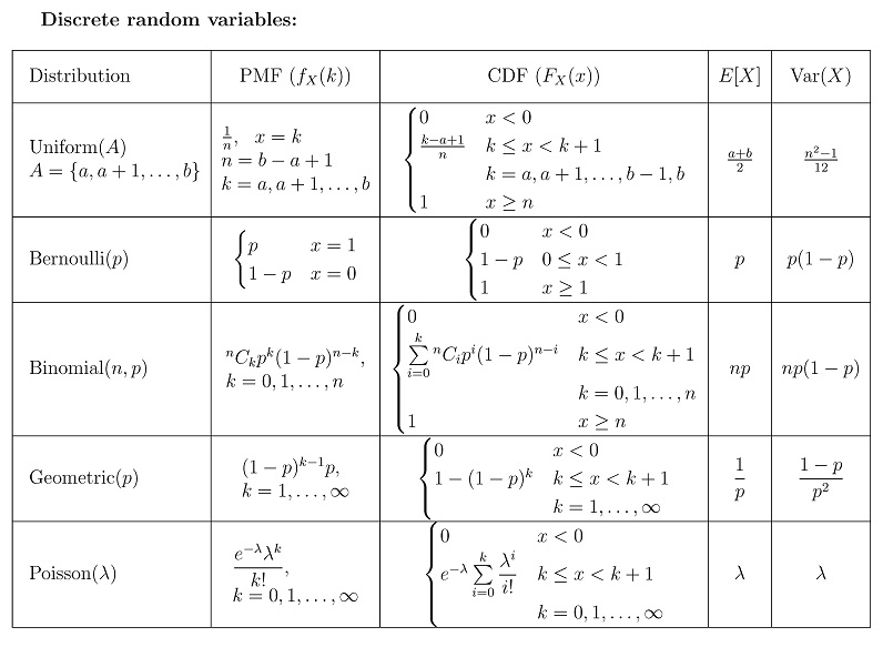
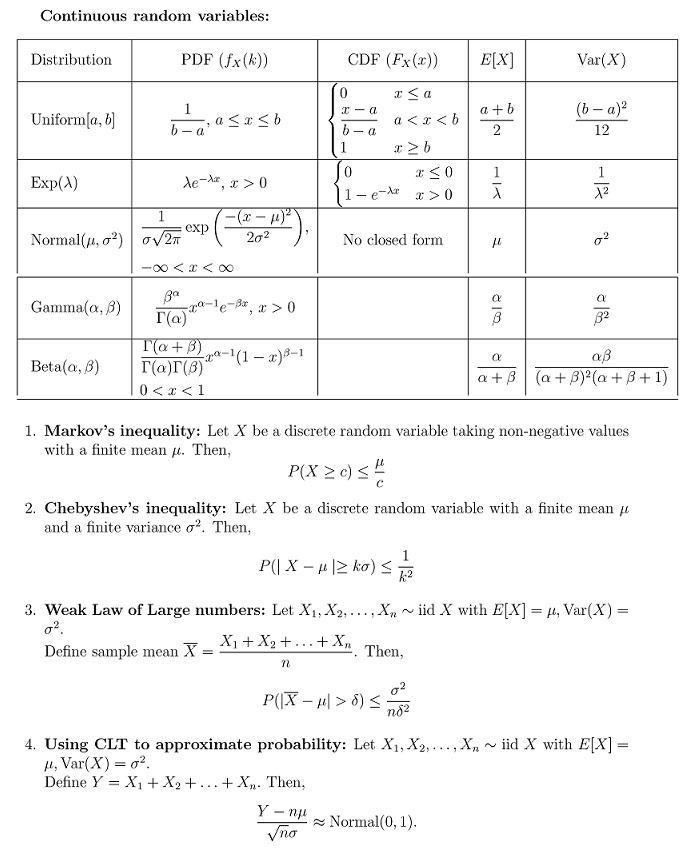
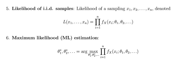
Useful Data has been mentioned above.
This data attachment is just for a reference & not for an evaluation.

Q2MSQ2 marksselect all that apply

Which of the following statements accurately describes the key difference between classification and regression models?

In classification, the output variable is continuous and real-valued, while inregression, it is categorical.
Regression models are used for predicting probabilities, whereas classificationmodels focus on predicting absolute values.
Classification models aim to find decision boundaries to separate data intoclasses, while regression models seek to predict a numeric value.
In regression, the commonly used loss function is mean squared error, whilein classification, 0 -1 loss is typically employed.

Comprehension passage - the questions below it refer to this

Based on the above data, answer the given subquestions. question figure

Q3SA2 marks

Your numeric answer:

Q4SA1 mark

Your numeric answer:

Q5MCQ3 marks

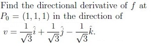
b1 − b2 + b3 = 0
b1 + b2 + b3 = 0
2b1 − b2 + b3 = 0
2b1 + b2 + b3 = 0

Q6MCQ3 marks

A consumer wants to maximize his utility subject to some constraints. He consumes two goods g1 and g2 and the utility function is the sum of g1 and g2. His budget is Rs.100. The per unit price of goods g1 and g2 are Rs.3 and Rs.4 respectively. Chose the correct optimization problem.

Q7MSQ4 marksselect all that apply

A − I (where I is the identity matrix of the same size) is also orthogonal.
Both AB and BA are orthogonal.
An and Bn are orthogonal for every n > 1.
A and B are also symmetric matrices.

Q8MSQ4 marksselect all that apply

Which of the following statements is/are true for a real symmetric matrix A?

AT A and AAT have the same rank.
AT A and AAT have the same eigenvalues
AT A and AAT have the same eigenvectors.
AT A and AAT have the same singular values.

Q9MSQ3 marksselect all that apply

Which of the following matrices is/are Unitary but not Hermitian?

Q10MSQ3 marksselect all that apply

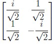
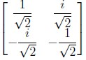
Which among the following is true for PCA?

The first principal component represents the direction along which thevariance of the dataset is maximized.
The first principal component represents the direction along which thevariance of the dataset is minimized.
The first principal component is the eigenvector corresponding to the smallesteigenvalue of the covariance matrix.
The first principal component is the eigenvector corresponding to the largesteigenvalue of the covariance matrix.

Q11MSQ3 marksselect all that apply

Which of the following statements regarding gradient descent is/are correct?

If the step size is chosen as 1, we may “not always” arrive as close to theoptimal solution even after many number of iterations.
Solution obtained for optimization problem is the local minimum of itsobjective function.
Solution obtained for optimization problem is the global minimum of itsobjective function.
Gradient descent converges to the global optimum in the case of convexfunctions.
Gradient descent does not converge to the global optimum in the case ofconvex functions.

Q12MSQ3 marksselect all that apply

Suppose a fair coin is tossed twice. Let A denote the event that the first toss is a tail. Let B denote the event that the second toss is a tail. Let C denote the event that out of the first two tosses, either both are heads or both are tails. Which among the following options are true? Select all that apply.

A, B and C are independent.
A, B and C are dependent.
A, B and C are pairwise independent.
P(A) = P(B) = P(C) = 1/2

Q13SA2 marks

Your numeric answer:

Q14SA3 marks

Your numeric answer:

Q15SA3 marks

Your numeric answer:

Q16SA3 marks

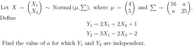
The average life (in years) of an electric bulb follows exponential distribution with parameter λ = 0.4. Using Weak Law of large numbers, find a lower bound on the probability that the mean life of a random sample of 50 such bulbs falls between 1.5 and 3.5 years. Enter your answer correct to three decimal places.

Your numeric answer:

Q17MCQ4 marks

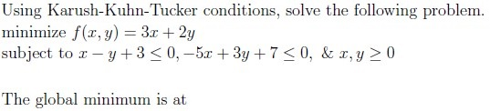
Answer key

Q1 (MCQ, 0 marks): A
Q2 (MSQ, 2 marks): C, D
Q3 (SA, 2 marks): 0
Q4 (SA, 1 marks): 7.44 to 7.52
Q5 (MCQ, 3 marks): C
Q6 (MCQ, 3 marks): A
Q7 (MSQ, 4 marks): B, C
Q8 (MSQ, 4 marks): A, B, D
Q9 (MSQ, 3 marks): A, D
Q10 (MSQ, 3 marks): A, D
Q11 (MSQ, 3 marks): A, B, D
Q12 (MSQ, 3 marks): B, C, D
Q13 (SA, 2 marks): 225
Q14 (SA, 3 marks): 1
Q15 (SA, 3 marks): 40
Q16 (SA, 3 marks): 0.870 to 0.880
Q17 (MCQ, 4 marks): C

Concepts this paper tests

Auto-generated summary from the source site. Handy as a checklist; the lessons above explain each idea from scratch.

Here’s a structured summary of the core topics, concepts, principles, and equations essential for the exam, followed by Mermaid knowledge graphs to visualize relationships.

1. Core Topics & Key Concepts

A. Probability & Statistics

1. Discrete & Continuous Distributions

Distribution	PMF/PDF	CDF	Mean ( $E[X]$ )	Variance ( $Var(X)$ )
Uniform (Discrete)	$f_X(k) = \frac{1}{n}, \quad k = a, a+1, \dots, b$	$F_X(x) = \frac{\lfloor x \rfloor - a + 1}{n}$	$\frac{a+b}{2}$	$\frac{n^2-1}{12}$
Bernoulli( $p$ )	$f_X(k) = p^k (1-p)^{1-k}, \quad k \in \{0,1\}$	$F_X(x) = (1-p) \cdot \mathbb{I}_{[0 \leq x < 1)} + \mathbb{I}_{x \geq 1}$	$p$	$p(1-p)$
Binomial( $n,p$ )	$f_X(k) = {}^nC_k p^k (1-p)^{n-k}, \quad k=0,1,\dots,n$	$F_X(x) = \sum_{i=0}^{\lfloor x \rfloor} {}^nC_i p^i (1-p)^{n-i}$	$np$	$np(1-p)$
Geometric( $p$ )	$f_X(k) = (1-p)^{k-1}p, \quad k=1,2,\dots$	$F_X(x) = 1 - (1-p)^{\lfloor x \rfloor}$	$\frac{1}{p}$	$\frac{1-p}{p^2}$
Poisson( $\lambda$ )	$f_X(k) = \frac{e^{-\lambda} \lambda^k}{k!}, \quad k=0,1,\dots$	$F_X(x) = e^{-\lambda} \sum_{i=0}^{\lfloor x \rfloor} \frac{\lambda^i}{i!}$	$\lambda$	$\lambda$
Uniform[ $a,b$ ]	$f_X(x) = \frac{1}{b-a}, \quad a \leq x \leq b$	$F_X(x) = \frac{x-a}{b-a} \cdot \mathbb{I}_{[a \leq x < b]} + \mathbb{I}_{x \geq b}$	$\frac{a+b}{2}$	$\frac{(b-a)^2}{12}$
Exponential( $\lambda$ )	$f_X(x) = \lambda e^{-\lambda x}, \quad x \geq 0$	$F_X(x) = 1 - e^{-\lambda x}$	$\frac{1}{\lambda}$	$\frac{1}{\lambda^2}$
Normal( $\mu, \sigma^2$ )	$f_X(x) = \frac{1}{\sigma \sqrt{2\pi}} e^{-\frac{(x-\mu)^2}{2\sigma^2}}$	No closed form	$\mu$	$\sigma^2$

2. Inequalities & Theorems

Markov’s Inequality:

P(X \geq c) \leq \frac{E[X]}{c}, \quad c > 0

Chebyshev’s Inequality:

P(|X - \mu| \geq k\sigma) \leq \frac{1}{k^2}

Weak Law of Large Numbers (WLLN):

P(|\overline{X} - \mu| > \delta) \leq \frac{\sigma^2}{n\delta^2}

Central Limit Theorem (CLT):

\frac{Y - n\mu}{\sqrt{n}\sigma} \approx \text{Normal}(0,1)

where $Y = X_1 + X_2 + \dots + X_n$ .

3. Likelihood & MLE

Likelihood Function:

L(\theta) = \prod_{i=1}^n f_X(x_i; \theta)

Maximum Likelihood Estimation (MLE):

\theta^* = \arg \max_\theta L(\theta)

B. Linear Algebra

1. Matrix Properties

Orthogonal Matrices:
- $A^T A = I$
- $\det(A) = \pm 1$
- Eigenvalues satisfy $|\lambda| = 1$ .
- If $A, B$ are orthogonal, then $AB$ is orthogonal.
Symmetric Matrices:
- $A = A^T$
- Eigenvalues are real.
- $A^T A$ and $AA^T$ have the same:
  - Rank
  - Eigenvalues
  - Singular values
Unitary Matrices:
- $U^H U = I$ (where $U^H$ is the conjugate transpose).
- Not necessarily Hermitian.

2. Linear Systems & Rank

Consistency Condition: For $A \mathbf{x} = \mathbf{b}$ to have a solution, $\mathbf{b}$ must lie in the column space of $A$ .
- Example: For the given matrix $A$ , the condition was $2b_1 - b_2 + b_3 = 0$ .

C. Optimization

1. Gradient Descent

Update Rule:

\theta_{t+1} = \theta_t - \eta \nabla f(\theta_t)

Properties:
- Converges to local minimum (not necessarily global).
- For convex functions, it converges to the global optimum.
- Step size ( $\eta$ ) affects convergence.

2. Karush-Kuhn-Tucker (KKT) Conditions

For constrained optimization:

\begin{align*} \text{Primal Feasibility: } & g_i(x) \leq 0, \quad h_j(x) = 0, \\ \text{Dual Feasibility: } & \lambda_i \geq 0, \\ \text{Complementary Slackness: } & \lambda_i g_i(x) = 0, \\ \text{Stationarity: } & \nabla f(x) + \sum \lambda_i \nabla g_i(x) + \sum \mu_j \nabla h_j(x) = 0. \end{align*}

D. Multivariable Calculus

1. Gradients & Directional Derivatives

Gradient:

\nabla f = \left( \frac{\partial f}{\partial x}, \frac{\partial f}{\partial y}, \frac{\partial f}{\partial z} \right)

Directional Derivative:

D_{\mathbf{v}} f(\mathbf{p}) = \nabla f(\mathbf{p}) \cdot \mathbf{v}

Maximum Rate of Change:

\|\nabla f\| = \sqrt{\left( \frac{\partial f}{\partial x} \right)^2 + \left( \frac{\partial f}{\partial y} \right)^2 + \left( \frac{\partial f}{\partial z} \right)^2}

2. Optimization Problems

Example: Minimize $f(x,y) = 3x + 2y$ subject to:

\begin{align*} x - y + 3 &\leq 0, \\ -5x + 3y + 7 &\leq 0, \\ x, y &\geq 0. \end{align*}

Solution: $(8, 11)$ .

E. Machine Learning Foundations

1. Classification vs. Regression

Aspect	Classification	Regression
Output	Categorical (discrete)	Continuous (real-valued)
Goal	Find decision boundaries	Predict numeric values
Loss Function	0-1 Loss, Cross-Entropy	Mean Squared Error (MSE)

2. Principal Component Analysis (PCA)

First Principal Component:
- Direction of maximum variance.
- Eigenvector corresponding to the largest eigenvalue of the covariance matrix.

2. Key Equations

Probability & Statistics

PMF/PDF/CDF for all distributions (see table above).
Markov’s Inequality:

P(X \geq c) \leq \frac{E[X]}{c}

Chebyshev’s Inequality:

P(|X - \mu| \geq k\sigma) \leq \frac{1}{k^2}

WLLN:

P(|\overline{X} - \mu| > \delta) \leq \frac{\sigma^2}{n\delta^2}

CLT:

\frac{Y - n\mu}{\sqrt{n}\sigma} \approx N(0,1)

Linear Algebra

Orthogonal Matrix:

A^T A = I

Eigenvalues of Symmetric Matrices:

\det(A - \lambda I) = 0

Rank of $A^T A$ and $AA^T$ :

\text{rank}(A^T A) = \text{rank}(AA^T) = \text{rank}(A)

Optimization

Gradient Descent Update:

\theta_{t+1} = \theta_t - \eta \nabla f(\theta_t)

KKT Conditions:

\begin{align*} \nabla f(x) + \sum \lambda_i \nabla g_i(x) &= 0, \\ \lambda_i g_i(x) &= 0, \quad \lambda_i \geq 0. \end{align*}

Multivariable Calculus

Gradient:

\nabla f = \left( \frac{\partial f}{\partial x}, \frac{\partial f}{\partial y}, \frac{\partial f}{\partial z} \right)

Directional Derivative:

D_{\mathbf{v}} f(\mathbf{p}) = \nabla f(\mathbf{p}) \cdot \mathbf{v}

Graph 2: Linear Algebra

Graph 3: Optimization

Graph 4: Machine Learning

Graph 5: Multivariable Calculus

This summary covers all essential topics, equations, and relationships for the exam.