Home / Past papers / MLF Quiz 1 / this paper
IIT M IMPROVEMENT AN EXAM QIB4 26 Oct - 26 Oct 2025
- Regression
- Classification
- Clustering
- Dimensionality Reduction













- No
- Yes
- Insufficient information to answer the question
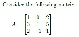
- {(1, 0, 2), (0, 1,−1)}
- {(1, 0, 2), (0, 1,−1), (0, 0,−1)}
- {(1, 0, 2), (0,−1, 1), (0,−1,−4)}
- {(0, 1,−1), (0, 0,−4)}
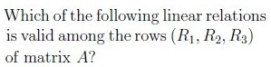



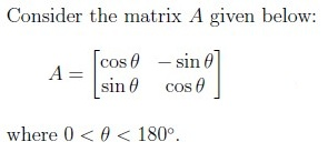
- A is an orthogonal matrix
- A is invertible
- A is symmetric
- A does not have real eigenvalues
- A has two distinct real eigenvalues
- A has two real eigenvalues, not necessarily distinct
- True
- False
- True
- False
- True
- False


- (A)
- (B)
Answer key
- Q1 (MCQ, 1 marks): B
- Q2 (MCQ, 3 marks): A
- Q3 (MSQ, 2 marks): B, C, D
- Q4 (SA, 3 marks): 72
- Q5 (SA, 3 marks): 1024
- Q6 (SA, 2 marks): 0
- Q7 (MCQ, 3 marks): A
- Q8 (MCQ, 2 marks): A
- Q9 (MCQ, 3 marks): B
- Q10 (MCQ, 2 marks): C
- Q11 (MSQ, 2 marks): A, B
- Q12 (MCQ, 3 marks): A
- Q13 (MCQ, 2 marks): B
- Q14 (MCQ, 1 marks): A
- Q15 (MCQ, 2 marks): B
- Q16 (MCQ, 2 marks): A
- Q17 (SA, 2 marks): 1
- Q18 (MCQ, 2 marks): A
Concepts this paper tests
Auto-generated summary from the source site. Handy as a checklist; the lessons above explain each idea from scratch.
Here’s a structured summary of core topics, concepts, principles, and equations for the Diploma-Level Machine Learning Foundations (Computer-Based Exam), along with Mermaid knowledge graphs to visualize relationships.
1. Core Topics & Concepts
A. Machine Learning Fundamentals
Supervised Learning
Classification (e.g., loan approval based on features like income, credit score).
- Algorithms: Logistic Regression, Decision Trees, SVM.
- Loss functions: Cross-entropy, Hinge loss.
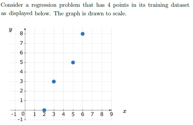
Regression (e.g., polynomial regression for quadratic models).
- Algorithms: Linear Regression, Polynomial Regression, Ridge/Lasso.
Loss functions: Mean Squared Error (MSE).
- Equation:
Least Squares Method for parameter estimation (θ₀, θ₁, θ₂ in ).
- Closed-form solution (Normal Equation):
Model Evaluation:
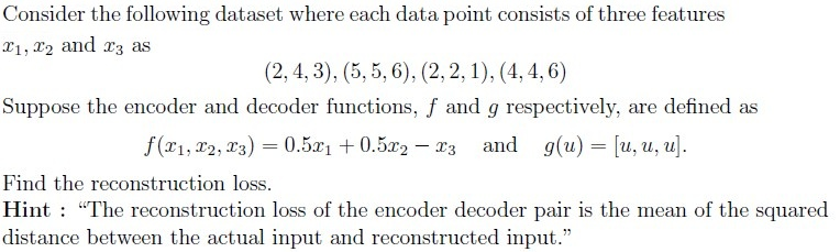
- Squared loss, reconstruction loss (e.g., autoencoders).
- Overfitting/underfitting.
Unsupervised Learning
- Clustering (e.g., K-Means, Hierarchical Clustering).
Dimensionality Reduction (e.g., PCA, Autoencoders).
- Autoencoder loss (reconstruction loss):
where = encoder, = decoder.
Key Distinctions:
- Classification vs. Regression vs. Clustering vs. Dimensionality Reduction.
B. Linear Algebra
Vectors
- Orthogonality: Two vectors and are orthogonal if .
- Linear Independence: Vectors are linearly independent if no vector can be written as a linear combination of others.
- Projection: Projection of onto :
- Parallel/Collinear Vectors: Vectors are parallel if one is a scalar multiple of the other.
Matrices
Eigenvalues/Eigenvectors:
- , where = eigenvalue, = eigenvector.
Properties:
- Sum of columns = zero vector ⇒ is an eigenvalue.
- Real symmetric matrices have real eigenvalues.
- Orthogonal matrices: (eigenvalues have magnitude 1).
Diagonalizability:
- A matrix is diagonalizable if it has linearly independent eigenvectors (not necessarily distinct eigenvalues).
Determinant:
- for a matrix where all non-zero vectors are eigenvectors with eigenvalue : .
Row Space/Basis:
- Row space of : Span of its rows.
- Basis: Linearly independent rows that span the row space.
Linear Relations:
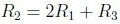
- Example: (from matrix rows).
Special Matrices
Orthogonal Matrices: .
- Example: Rotation matrix:
Eigenvalues: (complex if ).
- Symmetric Matrices: .
C. Calculus & Optimization
Linear Approximation
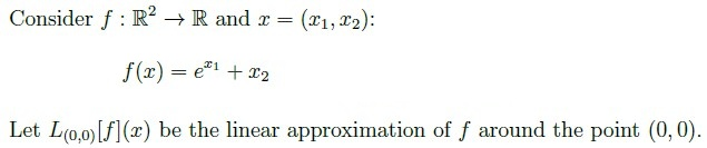
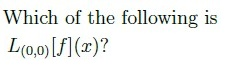
- For , the linear approximation at :
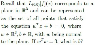
- Example for at :
- Plane Equation: , where is the normal vector.
Gradient Descent
- Update rule for regression:
D. Geometry
Contour Plots
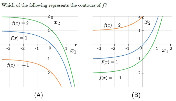
- Visualizing level sets of .
- Example: Contours of are horizontal shifts of exponential curves.
2. Key Equations
| Topic | Equation |
|---|---|
| Polynomial Regression | |
| Least Squares | |
| MSE Loss | |
| Reconstruction Loss | |
| Eigenvalue Equation | |
| Projection | |
| Linear Approximation | |
| Rotation Matrix | |
| Determinant of | (if all vectors are eigenvectors with eigenvalue ) |
Graph 2: Linear Algebra Concepts
Graph 3: Calculus & Optimization
Graph 4: Relationships Between Topics
4. Exam-Specific Tips
Polynomial Regression:
- For , construct the design matrix with columns and solve .
Eigenvalues/Eigenvectors:
- If all non-zero vectors are eigenvectors with eigenvalue , the matrix is , so .
Linear Approximation:
- For , compute gradients at :
So, .
Reconstruction Loss:
- Encode each data point, decode it, and compute the mean squared distance from the original.
Orthogonal Matrices:
- Rotation matrices are orthogonal and have eigenvalues , which are complex unless or .
Basis for Row Space:
- Perform row reduction (Gaussian elimination) to find linearly independent rows.