Home / Past papers / MLF End Term / this paper

IIT M IMPROVEMENT FN EXAM QDD1 01 Sep - 01 Sep 2024

MLF End Term14 questions40 marks6 SA · 5 MSQ · 3 MCQImprovement / forenoon / QDD1

Elapsed 00:00

Comprehension passage - the questions below it refer to this

A company produces two types of products P1 and P2. The cost price per unit of P1 and P2 are ₹2 and ₹3, respectively. The production process requires two types of resources: labor hours and machine hours. Each unit of p1 requires 2 labor hours and 1 machine hour, while each unit of P2 requires 1 labor hour and 3 machine hours. The company has constraints on the availability of labor and machine hours, which are 80 and 90 hours, respectively. Use the above information to answer the given sub-questions.

Q1MCQ2 marks

Choose the correct Primal optimization problem from the following.

Q2SA3 marks

Find the minimum cost price of the products.

Your numeric answer:

Q3MSQ3 marksselect all that apply

A circular park with one side boundary is a circle of radius of 200 meters andanother side boundary is a circle of radius of 300 meters, both centered at the origin.
City district defined by the region above the x-axis within a radius of 10 milesfrom the origin, forming a semicircle.
A triangular region with vertices at (0, 0), (1, 0), and (0, 1).
A path consisting of two connected line segments (forming the boundaries ofthe path on either sides) formed a “V” shape with vertices at (0, 0), (2, 2), and (2, 0)

Q4MSQ3 marksselect all that apply

Which of the following options is/are true?

Q5SA3 marks

A farmer has 120 meters of fencing and wants to fence off a rectangular field that borders a straight river. The farmer does not need to fence along the river. Find the maximum possible fenced area of the field.

Your numeric answer:

Q6SA3 marks

Suppose a random variable X has a mean μ of 70 and a standard deviation σ of 8. Using Chebyshev’s inequality, determine the maximum probability that X will deviate from the mean by more than 16 units. Enter the answer correct to two decimal places.

Your numeric answer:

Q7SA3 marks

Your numeric answer:

Q8SA3 marks

Your numeric answer:

Q9MSQ4 marksselect all that apply

Consider a square matrix A of order 3 such that trace(A) = 3 and det(A) = 2. If 1 is an eigenvalue of A, then which of the following options is/are true?

Matrix A is symmetric matrix.
Matrix A is Hermitian matrix.
1 + i is an eigenvalue of A.
2 − i is an eigenvalue of A.
Matrix A is diagonalizable.

Q10MSQ4 marksselect all that apply

Q11MSQ2 marksselect all that apply

Which of the following is/are true about PCA?

PCA will transform the original data set onto a lower dimension subspace suchthat the variance of the project is maximized.
PCA calculates the mean of each data set to determine its significance.
PCA can be used to reduce the dimensionality of the dataset.
PCA will transform the original data set onto a lower dimension subspace suchthat the reconstruction error is maximized.

Comprehension passage - the questions below it refer to this

Based on the above data, answer the given subquestions. question figure

Q12MCQ3 marks

Q13SA2 marks

Your numeric answer:

Q14MCQ2 marks

Answer key

Q1 (MCQ, 2 marks): B
Q2 (SA, 3 marks): 80
Q3 (MSQ, 3 marks): B, C
Q4 (MSQ, 3 marks): B, C, D
Q5 (SA, 3 marks): 1800
Q6 (SA, 3 marks): 0.25
Q7 (SA, 3 marks): 4.2
Q8 (SA, 3 marks): 0.262 to 0.268
Q9 (MSQ, 4 marks): C, E
Q10 (MSQ, 4 marks): B, C
Q11 (MSQ, 2 marks): A, C
Q12 (MCQ, 3 marks): B
Q13 (SA, 2 marks): 1
Q14 (MCQ, 2 marks): A

Concepts this paper tests

Auto-generated summary from the source site. Handy as a checklist; the lessons above explain each idea from scratch.

Here’s a structured summary of core topics, concepts, principles, and equations essential for the exam, followed by Mermaid knowledge graphs to visualize relationships.

Core Topics & Key Concepts

1. Linear Programming (Optimization)

Primal Problem Formulation:
- Objective: Minimize/maximize a linear function (e.g., cost/profit).
- Constraints: Linear inequalities (e.g., resource limits).
- Standard Form:

\text{Minimize } c^T x \quad \text{subject to } Ax \leq b, \, x \geq 0

Example (Q2, Q3):
- Objective: Minimize $2x + 3y$ (cost of P1 and P2).
- Constraints:

2x + y \leq 80 \quad (\text{labor hours}), \quad x + 3y \leq 90 \quad (\text{machine hours})

Solution: Use graphical method or simplex algorithm to find the feasible region’s vertices and evaluate the objective function.

Key Equations:
- Feasible Region: Intersection of all constraints.
- Optimal Solution: Vertex of the feasible region with the lowest/highest objective value.

2. Convex Sets & Functions

Convex Set:
- A set $S$ is convex if for any $x, y \in S$ and $\lambda \in [0,1]$ , $\lambda x + (1-\lambda)y \in S$ .
- Examples (Q4):
  - Semicircle (convex).
  - Triangle (convex).
  - "V" shape (not convex unless filled).

Convex Function:
- A function $f$ is convex if for all $x, y$ and $\lambda \in [0,1]$ :

f(\lambda x + (1-\lambda)y) \leq \lambda f(x) + (1-\lambda)f(y)

Tests for Convexity (Q5):
- Quadratic Forms: $f(v) = v^T A v$ is convex if $A$ is positive semidefinite (eigenvalues $\geq 0$ ).
  - Example: $A = \begin{bmatrix} 2 & 1 \\ 1 & 1 \end{bmatrix}$ (eigenvalues: $1.5 \pm 0.5\sqrt{5} > 0$ ).
- Hessian Matrix: For $f(x, y) = x^2 + y^2 + 3$ , the Hessian is $I$ (positive definite).
- Product of Convex Functions: Not necessarily convex (e.g., $f(x) = (x^2 - 3x + 2)(x^2 - 7x + 12)$ is not convex).

Key Equations:
- Hessian for $f(x, y)$ :

H = \begin{bmatrix} \frac{\partial^2 f}{\partial x^2} & \frac{\partial^2 f}{\partial x \partial y} \\ \frac{\partial^2 f}{\partial y \partial x} & \frac{\partial^2 f}{\partial y^2} \end{bmatrix}

Positive Semidefinite Check: All eigenvalues of $H \geq 0$ .

3. Optimization in Geometry

Maximizing Area (Q6):
- Problem: Fence a rectangular area along a river (3 sides fenced) with 120m of fencing.
- Solution:
  - Let width = $w$ , length = $L$ .
  - Constraint: $2w + L = 120$ .
  - Area: $A = w \times L = w(120 - 2w)$ .
  - Maximize: Find vertex of parabola $A = -2w^2 + 120w$ .
  - Optimal: $w = 30$ , $L = 60$ , $A = 1800$ .

Key Equation:

A = -2w^2 + 120w \quad \text{(Quadratic optimization)}

4. Probability & Statistics

Chebyshev’s Inequality (Q7):
- For any random variable $X$ with mean $\mu$ and variance $\sigma^2$ :

P(|X - \mu| \geq k\sigma) \leq \frac{1}{k^2}

Example: $\mu = 70$ , $\sigma = 8$ , $k = 2$ :

P(|X - 70| \geq 16) \leq \frac{1}{4} = 0.25

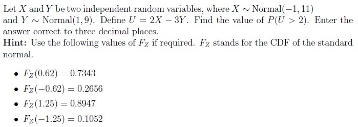
Linear Combinations of Normals (Q9):
- If $X \sim N(\mu_X, \sigma_X^2)$ and $Y \sim N(\mu_Y, \sigma_Y^2)$ are independent, then:

U = aX + bY \sim N(a\mu_X + b\mu_Y, a^2\sigma_X^2 + b^2\sigma_Y^2)

Example: $U = 2X - 3Y$ where $X \sim N(-1, 11)$ , $Y \sim N(1, 9)$ :

U \sim N(2(-1) - 3(1), 4(11) + 9(9)) = N(-5, 125)

Standardize to find $P(U > 2)$ :

P\left(Z > \frac{2 - (-5)}{\sqrt{125}}\right) = P(Z > 0.62) = 0.2656

Key Equations:

Z = \frac{U - \mu_U}{\sigma_U}, \quad P(U > u) = 1 - F_Z\left(\frac{u - \mu_U}{\sigma_U}\right)

5. Linear Regression (Q8)

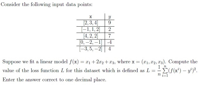
Loss Function (MSE):

L = \frac{1}{n} \sum_{i=1}^n (f(x_i) - y_i)^2

Example: For $f(x) = x_1 + 2x_2 + x_3$ and given data points, compute $L = 4.2$ .

Key Steps:
1. Predict $\hat{y}_i = f(x_i)$ .
2. Compute squared errors $(\hat{y}_i - y_i)^2$ .
3. Average over all points.

6. Linear Algebra (Q10, Q15)

Eigenvalues & Diagonalizability (Q10):
- Given: $\text{trace}(A) = 3$ , $\det(A) = 2$ , eigenvalue $\lambda_1 = 1$ .
- Find Other Eigenvalues:

\lambda_1 + \lambda_2 + \lambda_3 = 3 \implies \lambda_2 + \lambda_3 = 2

\lambda_1 \lambda_2 \lambda_3 = 2 \implies \lambda_2 \lambda_3 = 2

Solutions: $\lambda_2, \lambda_3 = 1 \pm i$ (complex conjugate pair).
- Diagonalizable: Yes, if $A$ has $n$ linearly independent eigenvectors (true for distinct eigenvalues).

Nullspace (Q15):
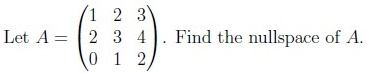
- For matrix $A$ , solve $A x = 0$ .
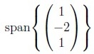
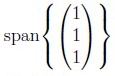
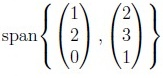
- Example: Nullspace of $A$ is $\text{span}\{\begin{pmatrix} 1 \\ -2 \\ 1 \end{pmatrix}\}$ .

Key Equations:

\text{Characteristic polynomial: } \det(A - \lambda I) = 0

7. Principal Component Analysis (PCA) (Q12)

Goal: Reduce dimensionality while maximizing variance.
Steps:
1. Center the data (subtract mean).
2. Compute covariance matrix $S$ .
3. Find eigenvalues/eigenvectors of $S$ .
4. Project data onto top $k$ eigenvectors (principal components).
Key Points:
- Variance Maximization: PCA selects directions with highest variance.
- Reconstruction Error: Minimized (not maximized).

8. Probability Distributions (Q13, Q14)

Joint & Conditional Distributions (Q13, Q14):
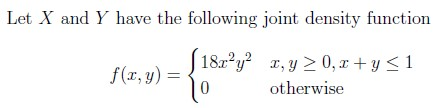
- Joint PDF: $f(x, y) = 18x^2y^2$ for $x, y \geq 0$ , $x + y \leq 1$ .
- Conditional PDF:

f_{X|Y}(x|y) = \frac{f(x, y)}{f_Y(y)} = \frac{18x^2y^2}{\int_0^{1-y} 18x^2y^2 \, dx} = \frac{3x^2}{(1-y)^3}, \quad 0 < x < 1-y

Conditional Probability (Q14):

P\left(X < \frac{1}{2} \mid Y = \frac{1}{2}\right) = \int_0^{1/2} f_{X|Y}\left(x \mid \frac{1}{2}\right) \, dx = 1

Key Equations:

f_Y(y) = \int_{-\infty}^\infty f(x, y) \, dx, \quad f_{X|Y}(x|y) = \frac{f(x, y)}{f_Y(y)}

9. Multivariate Optimization (Q11)

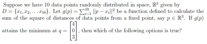
Minimizing Sum of Squared Distances:
- Problem: Minimize $g(p) = \sum_{i=1}^n \|p - x_i\|^2$ .
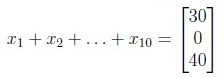
- Solution: The minimizer $q$ is the mean of the data points:

q = \frac{1}{n} \sum_{i=1}^n x_i

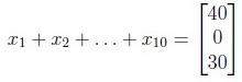
Example: Given $q = \begin{pmatrix} 4 \\ 0 \\ 3 \end{pmatrix}$ , the sum of data points is $10q = \begin{pmatrix} 40 \\ 0 \\ 30 \end{pmatrix}$ .

IIT M IMPROVEMENT FN EXAM QDD1 01 Sep - 01 Sep 2024

Answer key

Concepts this paper tests

Core Topics & Key Concepts

1. Linear Programming (Optimization)

2. Convex Sets & Functions

3. Optimization in Geometry

4. Probability & Statistics

5. Linear Regression (Q8)

6. Linear Algebra (Q10, Q15)

7. Principal Component Analysis (PCA) (Q12)

8. Probability Distributions (Q13, Q14)

9. Multivariate Optimization (Q11)

Graph 2: Probability & Statistics

Graph 3: Linear Algebra & PCA

Graph 4: Regression & Geometry